
1
Ch. 14 Subband Coding
Introduction &
Multirate Background
Next

2
Introduction
Given signal x[n] to compress…
Idea
: Split signal into M signals x
1
[n], x
2
[n], … , x
M
[n]
such that each signal can be more easily/effectively compressed.
Goal
: signals x
1
[n], x
2
[n], … , x
M
[n] should be made such that
– Each x
i
[n] is uncorrelated…
• then using SQ on each is a viable (though still suboptimal) approach
–Some x
i
[n] have smaller dynamic range
• Then can use fewer bits for a given desired distortion
– Should be a clear way to exploit psychological effects (for audio and
video) or other effects that imply some x
i
[n] are more important
Next
3
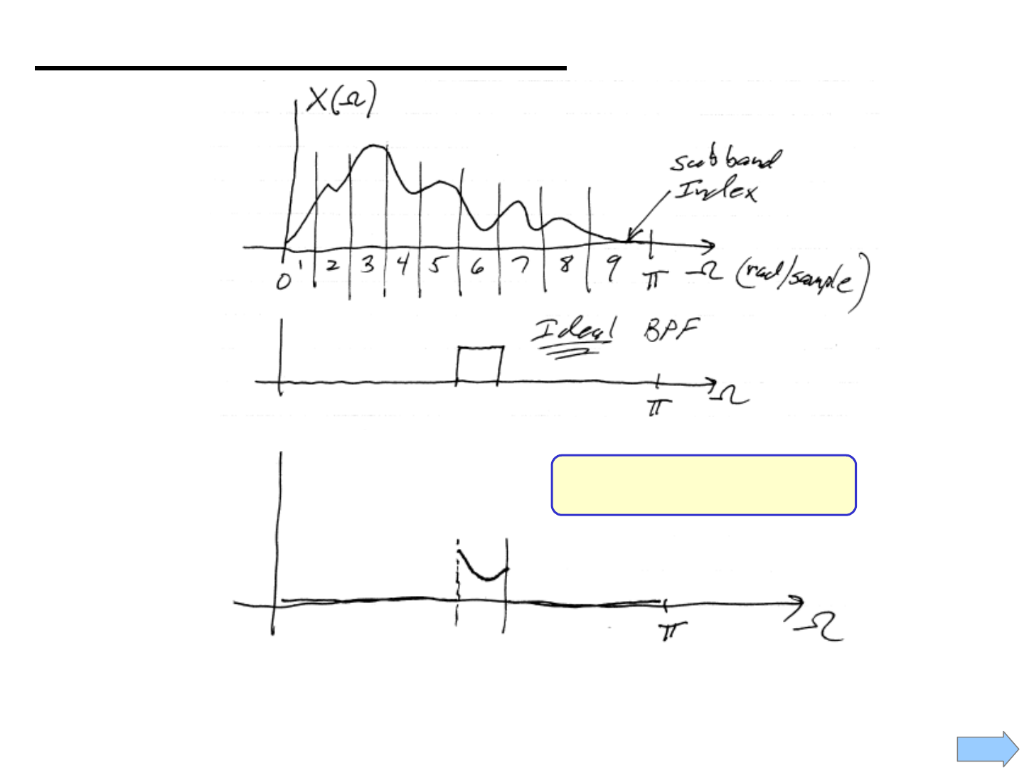
Illustration of Subbands
DTFT
of x[n]
H
6
(Ω)
X
6
(Ω)
Each x
i
[n] is called a
subband signal
[-π,0) is not shown
(Recall Symmetry)
Next

4
Motivational Form (Not Practical)
Compress
& Code
…
x[n]
x
1
[n]
x
M
[n]
Compress
& Code
M
U
X
bit
stream
bit
stream
D
E
M
U
X
De-Code
…
bit stream
bit
stream
Data Link
h
1
[n]
h
M
[n]
1
ˆ
[]
x
n
ˆ
[]
M
x
n
ˆ
[]
x
n
De-Code
Problems w/ This Form
• Output of each filter is at
input sampling rate
–Overallsample rate after
subband filters is M×F
s
• Can’t build Ideal BPFs
– Can’t reconstruct by just
adding together
• Inefficient to implement M
separate filters
Σ
Ideal
BPFs
…
Next

5
Fixing Sample Rate Problem: Multirate
Take a look at x
1
[n]
Ωπ-π
0
π/M
-π/M
X
1
(Ω)
This signal is oversampled
by a factor of M
(If it were not oversampled it would fill the entire -π to π)
To sample it slower by a factor of M… just throw away M-1 samples out of
every M samples (called “Decimation by M
”)…
h
1
[n]
x[n]
x
1
[0] x
1
[1] x
1
[2] x
1
[3] x
1
[4] x
1
[5] x
1
[6] x
1
[7] x
1
[8]
M = 3
h
1
[n]
x[n]
↓M
x
1
[0] x
1
[3] x
1
[6]
M = 3
Next

6
Now… we need someway at the decoder side to get back up to the original
sampling rate (called “Expansion by M
”)…
h
1
[n]
x[n]
↓M
M = 3
Code De-Code
Link
↑M
ˆˆˆ
[0] [3] [6]xxx"
ˆˆˆ
[0] 0 0 [3] 0 0 [6]xxx"
Has correct # samples/sec…
But can’t have those zeros!!!
A filter can “smooth out” the jumps due to the zeros (called “Interpolation
”)….
↑M
ˆˆˆ
[0] [3] [6]xxx"
ˆˆˆ
[0] 0 0 [3] 0 0 [6]xxx"
k
1
[n]
ˆˆˆˆˆˆˆ
[0][1][2][3][4][5][6]xxxxxxx"
Ideally:
Next

7
Subband Coding System
We can do a similar thing for all the other channels… and the result is:
Next

8
Roughly…What should the analysis filters look like?
Gaps will
result in
loss of info
Note: These are not true achievable shapes of filter frequency responses
Next

9
Subband Coding System Details
Encoding/Decoding Goals:
1. Choose methods matched to resulting channel characteristics
2. Allocate bit budget across the channels
Filter Design Goal: If we remove encode/decode… then we want our filters
to be designed so that output = input… this is called “Perfect Reconstruction
”.
Analysis Filters
must also provide frequency decomposition into
essentially non-overlapping subbands… should give “easy to code” signals
Synthesis Filters
are chosen to give the desired perfect reconstruction.
Their design will depend on the design of the analysis filters.
Multi-Rate Goal: properly decrease and then restore the sampling rate
Decimation
reduces each channel’s sample rate to keep the total analysis
filter bank’s output sample rate equal to the input sample rate
Interpolation
returns each channel to original rate before reconstruction
Next

10
To understand how filter banks work we need to understand:
• Effect of decimation on signal spectrum
• Effect of expansion on signal spectrum
• How to choose Analysis & Synthesis filters to achieve perfect
reconstruction (PR)
Next

11
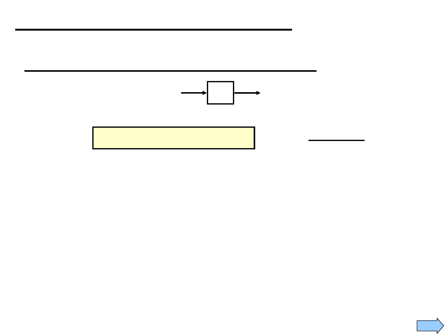
Decimation (Down Sampling)
Consider
H(Ω)
x[n]
y[n]
(sampled @ F
s
)
First let H(Ω) be an ideal
LPF w/ cut-off frequency Ω = π/2… “half-band filter”
Ω
π/2–π
H(Ω)
–π/2 π
Ideal Filter
for Illustration
Ω
π–π
X(Ω)
()
H
z
Ω
π–π π/2-π/2
Y(Ω)
Now… imagine what continuous-time signal would give y[n] if it were
sampled at F
s
:
Ω
π–π π/2-π/2
Y(Ω)
f
F
s
/2F
s
/4-F
s
/4-F
s
/2
So… if we sampled this CT signal at
half the original rate (@ F
s2
=F
s
/2)
then we would get this:
Ω
π-π
Y
2
(Ω)
f
F
s2
/2-F
s2
/2
Next

12
Ω
π–π
X(Ω)
↓2
()
H
z
–π
Ω
π/2–π
H(Ω)
–π/2 π
Ideal Filter
for Illustration
So… just looking at things in the DT domain with the sampling rate change
happening because of down-sampling… we should see the SAME thing:
In general… if the filter passes only in the range Ω∈[-π/M, π/M] we can
downsample by M
Now… all of this was based on “intuition” and for an Ideal
LPF… We need to
do a detailed analysis….
Ω
π–π
Y(Ω)
Ω
π
W(Ω)
x[n] y[n] w[n]
Next
13
[] [ ] forwn yMn n Z=∈
M-Fold Decimation
[0] [0]
[1] [3]
[2] [6]
wx
wx
wx
=
=
=
#
For M=3
Decimation – Time-Domain Math View
↓M
y[n]
w[n]
Math Analysis of Decimation
To really understand what is happening we need to look in the
frequency domain…
Next

14
Notation:
)(
zz
)()(
)}({)()}({
MMM
zXzXzZx
↓↓↓
==
• Similar for DTFT
• Similar for Expansion
Q: What is X
(↓M)
(z) in terms of X(z)???
What do we expect????!!!!
Lower F
s
causes Spectral Replicas to Move to Lower Frequencies
Should look exactly like
sampling at a lower F
s
Thus… increased aliasing is possible!!!
To answer this we need to define a useful function (“comb” function):
∑∑
−
=
∞
−∞=
==−=
1
0
1
]mod[][][
M
m
mn
M
k
M
W
M
MnkMnnc
δδ
Call this ()…
This is like a DT
Fourier Series and is
easily verified!
m
036-3-6
1
C
3
(m)
M-Fold Decimation – Frequency-Domain
2/
j
M
M
We
π
Next

15
][][
][][
)(
nMcnMx
nMxnx
M
M
=
=
↓
Now… use the comb function to write decimation:
Doesn’t Really Do
Anything Here…
But Later it Will!!
Action of C
M
[n]
∑∑
∞
−∞=
−
−
=
↓
⎥
⎥
⎦
⎤
⎢
⎢
⎣
⎡
=
n
Mn
M
m
mn
M
z
M
zW
M
nxzX
/
1
0
)(
1
][)(
Now… take Z-Transform, using this form:
M-Fold Decimation – Frequency-Domain (cont.)
Now… take Z-Transform, using this form:
01 2
()
[0] [ ] [2 ]
() [][]
zn
M
M
n
xzxMz xMz
Xz xnMcnMz
−
∞
−
↓
=−∞
++ + +
=
∑
""
01
/
[0] 0 0 [ ] 0
[] []
nM
M
n
xz xMz
xnc nz
−
∞
−
=−∞
+++++ ++
=
∑
"" "
Next
16
()
)(
1
][
1
1
][)(
/1
1
0
1
0
/1
/
1
0
)(
Mm
M
M
m
z
M
mn
n
Mm
M
n
Mn
M
m
mn
M
z
M
zWX
M
zWnx
M
zW
M
nxzX
−
−
=
−
=
∞
−∞=
−
−
∞
−∞=
−
−
=
↓
∑
∑∑
∑∑
=
⎥
⎥
⎦
⎤
⎢
⎢
⎣
⎡
=
⎥
⎥
⎦
⎤
⎢
⎢
⎣
⎡
=
Now… just manipulate:
)(
1
)(
/1
1
0
)(
Mm
M
M
m
zz
M
zWX
M
zX
−
−
=
↓
∑
=
ZT of Decimated Signal is…
M-Fold Decimation – Frequency-Domain (cont.)
Next

17
Now to see a little better what this says… convert ZT to DTFT.
MjMj
ezez
//1
θθ
=⇒=
1. Axis-Scale X
f
(θ) to get X
f
(θ/M) – a stretch
2. Then shift by 2πm to get new replicas
Î Decimation Adds Spectral Replicas of Scaled DTFT
∑
−
=
↓
⎟
⎠
⎞
⎜
⎝
⎛
−
=
1
0
ff
)(
21
)(
M
m
M
M
m
X
M
X
πθ
θ
Mmjm
M
eW
/2
π
−−
=Also, by definition:
DTFT of Decimated Signal is…
Stretches
Spectrum
M-Fold Decimation – Frequency-Domain (cont.)
Recall: DTFT is the ZT evaluated on the unit circle:
Then we get….
Next

18
M = 3
0 π 2π 3π 4π 5π 6π 7π 8π 9π-π-2π-3π-4π-5π-6π-7π-8π-9π
±π/3
θ
X
f
(θ)
Original
0 π 2π 3π 4π 5π 6π 7π 8π 9π-π-2π-3π-4π-5π-6π-7π-8π-9π
X
f
(θ/3)
θ
m = 0
0 π 2π 3π 4π 5π 6π 7π 8π 9π-π-2π-3π-4π-5π-6π-7π-8π-9π
X
f
((θ-2π)/3)
θ
m = 1
0 π 2π 3π 4π 5π 6π 7π 8π 9π-π-2π-3π-4π-5π-6π-7π-8π-9π
X
f
((θ-4π)/3)
θ
m = 2
Example: DTFT for M-Fold Decimation
Next
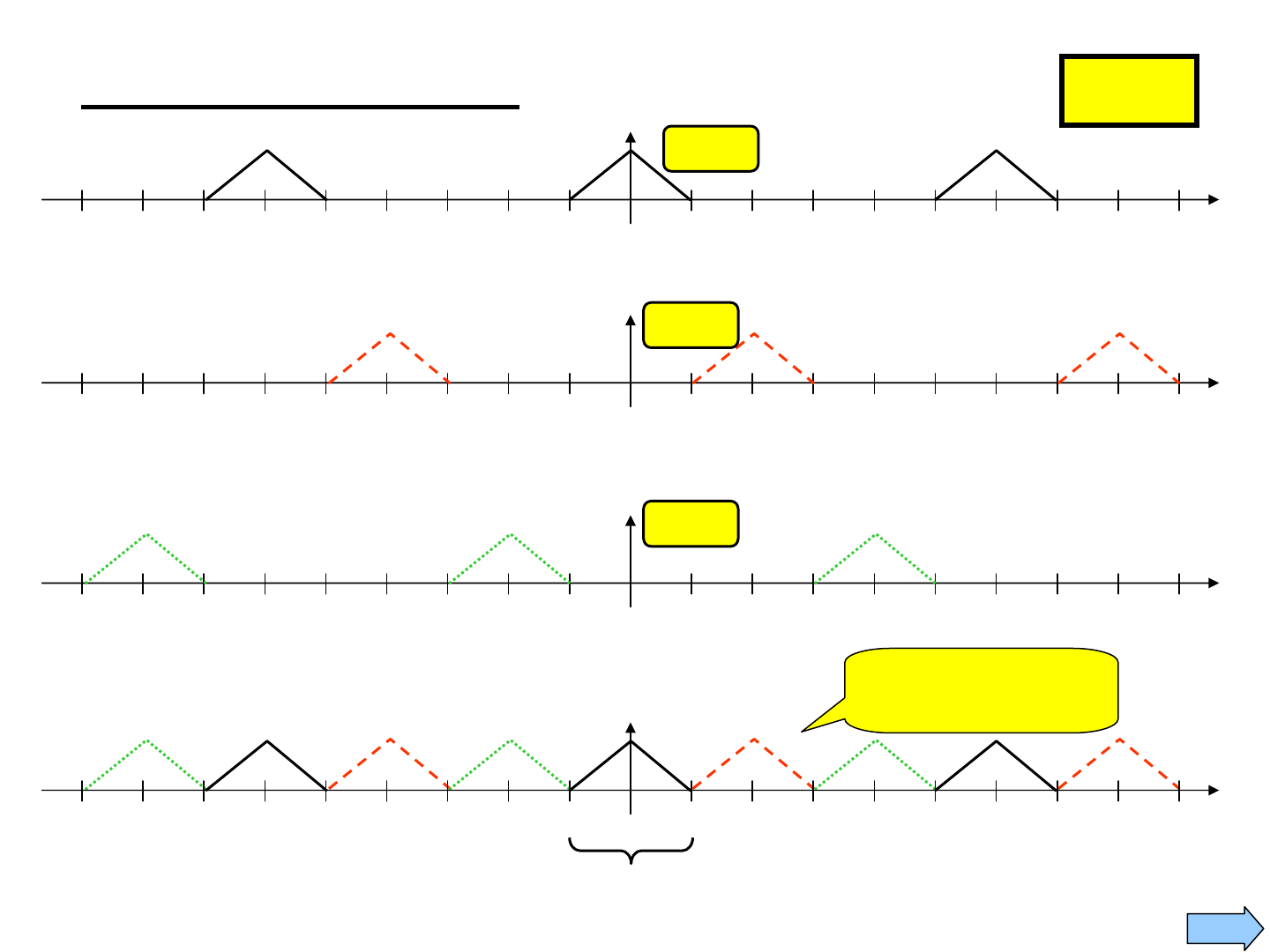
19
M = 3
0
π 2π 3π 4π 5π 6π 7π 8π 9π-π-2π-3π-4π-5π-6π-7π-8π-9π
X
f
(θ/3)
θ
m = 0
0 π 2π 3π 4π 5π 6π 7π 8π 9π-π-2π-3π-4π-5π-6π-7π-8π-9π
X
f
((θ-2π)/3)
θ
m = 1
0
π 2π 3π 4π 5π 6π 7π 8π 9π-π-2π-3π-4π-5π-6π-7π-8π-9π
X
f
((θ-4π)/3)
θ
m = 2
)(
f
)(
θ
M
MX
↓
0 π 2π 3π 4π 5π 6π 7π 8π 9π-π-2π-3π-4π-5π-6π-7π-8π-9π
θ
M × DTFT of
Decimated Signal
No Aliasing!!!
Example: Continued
Next

20
1. The M-decimated signal will have no aliasing… only if
the signal being decimated has:
MX /for 0)(
f
πθθ
>=
This makes complete sense from an
“ordinary” sampling theorem view point!!!
2. After M-decimating an M
th
-band signal, the spectrum of
the decimated signal will fill the [-π, π] band.
Such a signal is called
an “M
th
-Band Signal”
Example: Insights
Next

21
Although decimation changes the digital frequency of the
signal, the corresponding “physical” frequency is not
changed… as the following example shows:
↓3
x[n]
Fs
1
=60 MSPS
x
(↓3)
[n]
Fs
2
= 60/3
= 20 MSPS
0
π-π
θ
X
(↓3)
(θ)
0
f
2
2
s
F
2
2
s
F
−
-10
MHz
10
MHz
0
π-π
θ
X
f
(θ)
0
f
2
1
s
F
2
1
s
F
−
-10
MHz
10
MHz
Signal Still Occupies Same Physical Frequency
Note
Expansion
Also Has
No Effect
on Physical
Frequency
Effect on “Physical” Frequency
Next

22
Q: What is X
(↑L)
(z) in terms of X(z)???
What do we expect????!!!!
Certainly NOT the same as really sampling at a higher rate
because of the inserted zeros!!!
Frequency Domain analysis answers this!!!
)()(
)(
Lzz
L
zXzX =
↑
ZT of Expanded Signal is…
L-Fold Expansion – Frequency-Domain
02
1 zeros 1 zeros
[0] 0 0 [1] 0 0 [2]
L
L
LL
xz xz xz
−−
−−
=++ ++++ ++++"" "
() ()
() []
zn
LL
n
X
zxnz
∞
−
↑↑
=−∞
=
∑
[] ( )
Ln z L
n
xnz X z
∞
−
=−∞
==
∑
Next

23
Now to see a little better what this says… convert ZT to DTFT.
Recall: DTFT is the ZT evaluated on the unit circle:
θθ
jLLj
ezez =⇒=
DTFT of Decimated Signal is…
)()(
ff
)(
θθ
LXX
L
=
↑
Scrunches
Spectrum
L-Fold Expansion – Frequency-Domain (cont.)
Next
24
0 π 2π 3π 9π-π-2π-3π
)(
f
θ
X
θ
…
…
L = 3
θ
)(
f
θ
LX
0
π 2π 3π-π-2π-3π
…
…
π/3
-π/3
Expansion Causes Images
to Appear in the [-π,π] Range
…
θ
0 π 2π 3π-π-2π-3π
…
π/3
-π/3
Here’s what we’d have if we REALLY sampled
3 times as fast… No Images
!!!
Example: DTFT for L-Fold Expansion
Next

25
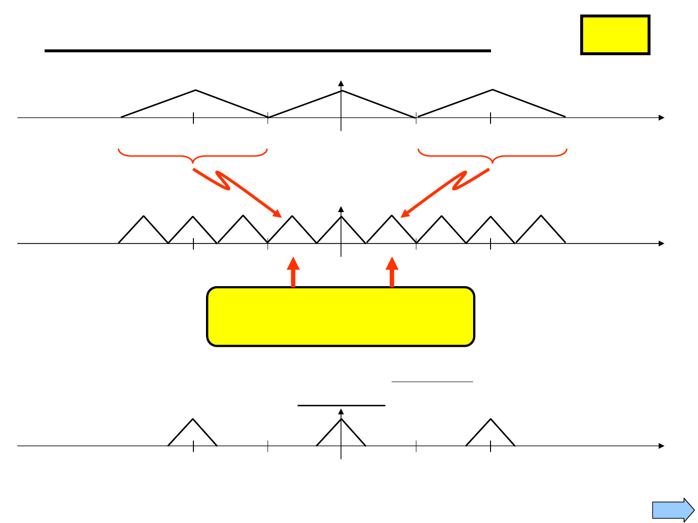
Effect of Non-Ideal Filters
Ω
π–π
X(Ω)
↓2
()
H
z
Ω
π/2–π
H(Ω)
–π/2 π
x[n] y[n] w[n]
Y(Ω)
Ω
π–π 2π–2π
Y((Ω-2π)/2)
Ω
Y(Ω/2)
Ω
π–π 2π–2π 4π-4π
0
–3π 3π
π–π 2π–2π 4π-4π
0
–3π 3π
Aliasing
Aliasing
W(Ω)
Ω
π–π 2π–2π 4π-4π
0
–3π 3π
Aliasing
Next

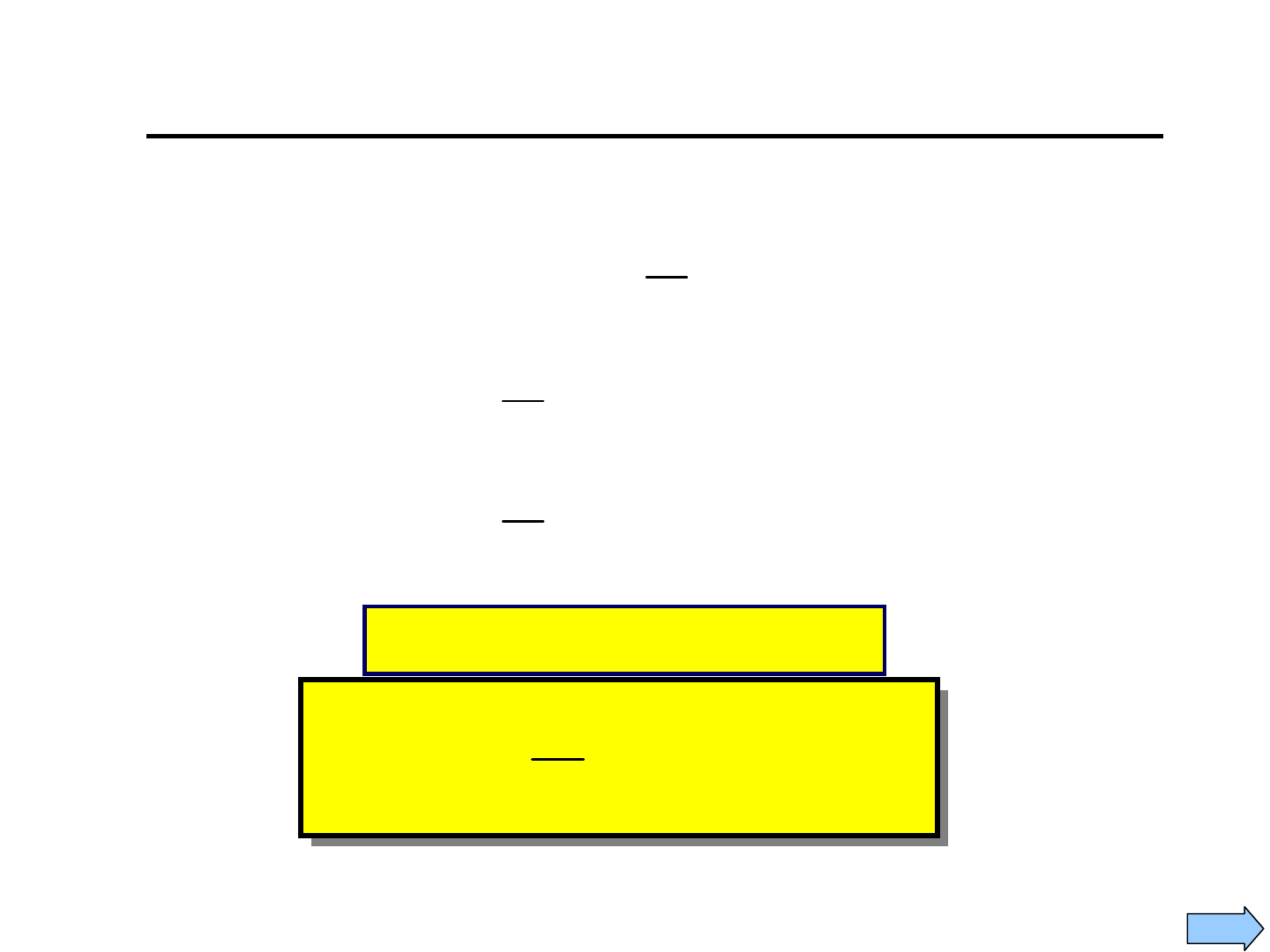
26
Summary
So… in practice we can change the rate of a signal… but there will always be some
error due to non-ideal filters (both in the case of downsampling and in the case of
upsampling).
Generally, we can design the filters to make these errors negligible …
BUT
… such filters are long FIR filters and that can lead to efficiency issues
Note
: Similar analyses can be done for
•HPF
followed by Decimation
• Interpolation followed by HPF
↓M
()H Ω
x[n] y[n] w[n]
↑M
()K
Ω
w[n] v[n] u[n]
1
0
12
()
M
m
m
WY
MM
π
−
=
Ω−
⎛⎞
Ω=
⎜⎟
⎝⎠
∑
() ()()YXHΩ= Ω Ω
w/ H(Ω) having a passband
width of π/M
() ()( )UKWM
Ω
=Ω Ω
w/ K(Ω) having a
passband width of π/M
End
