Adaptive stepsizes for recursive estimation with applications in

Mach Learn (2006) 65:167–198

DOI 10.1007/s10994-006-8365-9

Adaptive stepsizes for recursive estimation with

applications in approximate dynamic programming

Abraham P. George · Warren B. Powell

Received: 23 July 2004 / Revised: 8 March 2006 / Accepted: 8 March 2006 / Published online: 17 May 2006

Springer Science +Business Media, LLC 2006

Abstract We address the problem of determining optimal stepsizes for estimating param-

eters in the context of approximate dynamic programming. The sufﬁcient conditions for

convergence of the stepsize rules have been known for 50 years, but practical computational

work tends to use formulas with parameters that have to be tuned for speciﬁc applications.

The problem is that in most applications in dynamic programming, observations for estimat-

ing a value function typically come from a data series that can be initially highly transient.

The degree of transience affects the choice of stepsize parameters that produce the fastest

convergence. In addition, the degree of initial transience can vary widely among the value

function parameters for the same dynamic program. This paper reviews the literature on

deterministic and stochastic stepsize rules, and derives formulas for optimal stepsizes for

minimizing estimation error. This formula assumes certain parameters are known, and an

approximation is proposed for the case where the parameters are unknown. Experimental

work shows that the approximation provides faster convergence than other popular formulas.

Keywords Stochastic stepsize · Adaptive learning · Approximate dynamic programming ·

Kalman ﬁlter

In most approximate dynamic programming algorithms, values of future states of the system

are estimated in a sequential manner, where the old estimate of the value (¯v

n−1

) is smoothed

with a new estimate based on Monte Carlo sampling (

). The new estimate of the value is

obtained using one of the two equivalent forms,

¯v

= ¯v

n−1

− α

(¯v

n−1

−

) (1)

= (1 − α

)¯v

n−1

+ α

. (2)

Editor: Prasad Tadepalli

A. P. George (



)

W. B. Powell

Department of Operations Research and Financial Engineering,

Princeton University, Princeton, NJ 08544

e-mail: [email protected]

W. B. Powell

e-mail: [email protected]

Springer

168 Mach Learn (2006) 65:167–198

is a quantity between 0 and 1 and is commonly referred to as a stepsize. In other commu-

nities, it is known by different names, such as learning rate (machine learning), smoothing

constant (forecasting) or gain (signal processing). The size of α

governs the rate at which

new information is combined with the existing knowledge about the value of the state.

The usual choices of stepsizes used for updating estimates include constants or declining

stepsizes of the type 1/n. If the observations, {

}

n=1,2,...

, come from a stationary series,

then using 1/n means that ¯v

is an average of previous values and is optimal in the sense that

it produces the lowest variance unbiased estimator.

It is often the case in dynamic programming that the learning process goes through an

initial transient period where the estimate of the value either increases or decreases steadily

and then converges to a limit at an approximately geometric rate, which means that the

series of observations is no longer stationary. In such situations, either of these stepsize rules

(constant or declining) would give an inferior rate of convergence. Nonstationarity could arise

if the initial estimate is of poor quality, in the sense that it might be far from the true value,

but with more iterations, we move closer to the correct value. Alternatively, the physical

problem itself could be of a nonstationary nature and it might be hard to predict when the

estimate has actually approached the true value. This leaves open the question of the optimal

stepsize when the data that is observed is nonstationary.

In the literature, similar updating procedures are encountered in other ﬁelds besides ap-

proximate dynamic programming. In the stochastic approximation community, Eq. (1) is

employed in a variety of algorithms. An example is the stochastic gradient algorithm which

is used to estimate some value, such as the minimum of a function of a random variable,

where the exogenous data involves errors due to the stochastic nature of the problem. The

idea in stochastic approximation is to weight the increment at each update by a sequence

of decreasing gains or stepsizes whose rate of decrease is such that convergence is ensured

while removing the effects of noise.

The pioneering work in stochastic approximation can be found in Robbins and Monro

(1951) which describes a procedure to approximate the roots of a regression function which

demonstrates mean-squared convergence under certain conditions on the stepsizes. Kiefer

and Wolfowitz (1952) suggests a method which approximates the maximum of a regression

function with convergence in probability under more relaxed conditions on the stepsizes.

Blum (1954b) proves convergence with probability one for the multi-dimensional case of the

Robbins-Monro procedure under even weaker conditions. Pﬂug (1998) gives an overview of

some deterministic and adaptive stepsize rules used in stochastic approximation methods,

and brings out the drawbacks of using deterministic stepsize rules, whose performance is

largely dependent on the initial estimate. According to this survey, it could be advantageous

to use certain adaptive rules that enable the stepsizes to vary with information gathered during

the progress of the estimation procedure. The survey compares the different stepsize rules for

a stochastic approximation problem, but does not establish the superiority of any particular

rule over another. Spall (2003) (Section 4.4) discusses the choice of stepsize sequence that

would ensure fast convergence of the general stochastic approximation procedure.

In the ﬁeld of forecasting, the proceduredeﬁnedby Eq. (2) is termed exponential smoothing

and is widely used to predict future values of exogenous quantities such as random demands.

The original workin this area can be found in Brown (1959) and Holt et al. (1960). Forecasting

models for data with a trend component have also been developed. In most of the literature,

constant stepsizes are used (Brown, 1959; Holt et al., 1960; Winters, 1960), mainly because

they are easy to implement in large forecasting systems and may be tuned to work well for

speciﬁc problem classes. However, it has been shown that models with ﬁxed parameters

will demonstrate a lag if there are rapid changes in the mean of the observed data. There

Springer

Mach Learn (2006) 65:167–198 169

are several methods that monitor the forecasting process using the observed value of the

errors in the predictions with respect to the observations. For instance, Brown (1963), Trigg

(1964) and Gardner (1983) develop tracking signals that are functions of the errors in the

predictions. If the tracking signal falls outside of certain limits during the forecasting process,

either the parameters of the existing forecasting model are reset or a more suitable model is

used. Gardner (1985) reviews the research on exponential smoothing, comparing the various

stepsize rules that have been proposed in the forecasting community.

There are several techniques in the ﬁeld of reinforcement learning that use time-dependent

deterministic models to compute the stepsizes. Darken and Moody (1991) addresses the

problem of having the stepsizes evolve at different rates, depending on whether the learning

algorithm is required to search for the neighborhood of the right solution or to converge

quickly to the true value—the stepsize chosen is a deterministic function of the iteration

counter. These methods have the drawback that they are not able to adapt to differential rates

of convergence among the parameters.

A few techniques have been suggested which compute the stepsizes adaptively as a func-

tion of the errors in the predictions or estimates. Kesten (1958) suggests a stepsize method

which makes use of the notion that if consecutive errors in the estimate of the value of a

parameter obtained by the Robbins-Monro stochastic approximation method are of oppo-

site signs, then the estimate is in the vicinity of the true value and therefore the stepsize

should be reduced. An extension of this idea is found in Saridis (1970) where, in addition

to decrementing the stepsize for errors of opposite signs, it is suggested to increment the

stepsizes if the consecutive errors are of the same sign so that the estimate moves closer to

the optimal parameter value. Fabian (2004) suggests adjusting the estimate based on the sign

of the error alone, instead of incrementing (or decrementing) the estimate in proportion to

the magnitude of the error, which is desirable in cases where a large value of error is not

necessarily indicative of a large deviation of the estimate from the true value.

In signal processing and adaptive control applications, there have been several methods

proposed that use time-varying stepsize sequences to improve the speed of convergence

of ﬁlter coefﬁcients. The selection of the stepsizes is based on different criteria such as

the magnitude of the estimation error (Kwong, 1986), polarity of the successive samples

of estimation error (Harris, Chabries and Bishop, 1986) and the cross-correlation of the

estimation error with input data (Karni & Zeng, 1989; Shan & Kailath, 1988). Mikhael

et al. (1986) proposes methods that give the fastest speed of convergence in an attempt to

minimize the squared estimation error, but at the expense of large misadjustments in steady

state. Bouzeghoub et al. (2000) analyzes, using simulation examples, the ability of several

updating algorithms for tracking nonstationary processes. The review compares the different

approaches used by these algorithms to balance proper tracking and noise averaging.

Another approach that is adopted is to adjust the stepsizes by a correction term that is

a function of the gradient of the error measure that needs to be minimized. One of the

techniques that uses this idea is the delta-bar-delta learning rule, proposed in Jacobs (1988),

which decreases the stepsize exponentially or increases them linearly depending on whether

the consecutive errors are of similar signs or not, respectively. Decreasing the stepsizes

exponentiallyensures that they remain positivewhile decreasing them fastwhereas increasing

them linearly prevents them from increasing too fast. Benveniste, Metivier and Priouret

(1990) proposes an alternative version of the gradient adaptive stepsize algorithm within a

stochastic approximation formulation. Brossier (1992) uses this approach to solve several

problems in signal processing and provides supporting numerical data. Proofs of convergence

of this approach for the stepsizes are given in Kushner and Yang (1995). Variations of the

gradient adaptive stepsize schemes are also employed in other adaptive ﬁltering algorithms

Springer

170 Mach Learn (2006) 65:167–198

and signal processing applications in Sutton (1992), Mathews and Xie (1993), Douglas and

Mathews (1995), Douglas and Cichocki (1998) and Schraudolph (1999). The limitation of

most gradient adaptive stepsize methods is the use of a smoothing parameter for updating

the stepsize values. The ideal value of the smoothing parameter is problem dependent and

could vary with each coefﬁcient that needs to be estimated. This may not be tractable for

large problems where several thousands of parameters need to be estimated.

This paper makes the following contributions.

• We provide a review of the stepsize formulas that address nonstationarity from different

ﬁelds.

• We propose an adaptive formula for computing the optimal stepsizes which minimizes the

mean squared error of the prediction from the true value for the case where certain problem

parameters, speciﬁcally the variance and the bias, are known. This formula handles the

tradeoff between structural change and noise.

• For the case where the parameters are unknown, we develop a procedure for prediction

where the estimates are updated using approximations of the optimal stepsizes. The algo-

rithm that we propose has a single unitless parameter. Our claim is that this parameter does

not require tuning if chosen within a small range. We show that the algorithm gives robust

performance for values of the parameter in this range.

• We present an adaptation of the Kalman ﬁltering algorithm in the context of approximate

dynamic programming where the Kalman ﬁlter gain is treated as a stepsize for updating

value functions.

• We provide experimental evidence that illustrates the effectiveness of the optimal stepsize

algorithm for estimating a variety of scalar functions and also when employed in forward

dynamic programming algorithms to estimate value functions of resource states.

The paper is organizedasfollows. In Section 1, we consider the case where the observations

form a stationary series and illustrate the known results for optimal stepsizes. Section 2

discusses the issue of nonstationarity that could arise in estimation procedures and reviews

some stepsize rules that are commonly used for estimation in the presence of nonstationarity.

In Section 3, we derive an expression for optimal stepsizes for nonstationary data, where

optimality is deﬁned in the sense of minimizing the mean squared error. We present an

algorithmic procedure for parameter estimation that implements the optimal stepsize formula

for the case where the parameters are not known. In Section 4, we discuss our experimental

results. Section 5 provides concluding remarks.

1. Optimal stepsizes for stationary data

We deﬁne a stationary series as one for which the mean value is a constant over the iterations

and any deviation from the mean can be attributed to random noise that has zero expected

value. When we employ a stochastic approximation procedure to estimate the mean value of

a stationary series, we are guaranteed convergence under certain conditions on the stepsizes.

We state the result as follows,

Theorem 1. Let {α

}

n=1,2,...

be a sequence of stepsizes (0 ≤ α

≤ 1 ∀n = 1, 2,...) that

satisfy the following conditions:

∞



n=1

=∞ (3)

Springer

Mach Learn (2006) 65:167–198 171

∞



n=1

(α

)

< ∞ (4)

If {

}

n=1,2,...

is a sequence of independent and identically distributed random variables with

ﬁnite mean, θ, and variance, σ

, then the sequence, {

}

n=1,2,...

, deﬁned by the recursion,

(α

) = (1 − α

)

n−1

+ α

(5)

and with any deterministic initial value, converges to θ almost surely.

Robbins and Monro (1951) describes a more general version of this procedure, which is

proved to be convergent in Blum (1954a). Equation (3) ensures that the stepsizes are large

enough so that the process does not stall at an incorrect value. The condition given by Eq.

(4) is needed to dampen the effect of experimental errors and thereby control the variance of

the estimate.

Let θ be the true value of the quantity that we try to estimate. The observation at iteration

n can be expressed as

= θ +ε

, where ε

denotes the noise. The elements of the random

noise process, {ε

}

n=1,2,...

, can take values in . We assume that the noise sequence is serially

uncorrelated with zero mean and a constant, ﬁnite variance, σ

We pose the problem of ﬁnding the optimal stepsize as one of solving,

min

0≤α

≤1

E[(

(α

) − θ )

] (6)

For the case of stationary observations, we state the following well-known result:

Theorem 2. The optimal stepsizes that solve (6) are given by,

(α

)

∗

∀ n = 1, 2,... (7)

Given the sequence of observations, {

}

i=1,2,...,n

, which has a static mean, it can be shown

that the sample mean, (

)

∗



i=1

, is the best linear unbiased estimator (BLUE)

of the true population mean (Kmenta, 1997), Section 6.2). It can be shown that in certain

cases a biased estimator can give a lower variance than the sample mean (Spall, 2003),

p. [334], however we limit ourselves to estimators that are unbiased. In a setting where the

observations are made sequentially, the sample mean can be computed recursively (see Young

(1984)) as a weighted combination of the current observation and the previous estimate,

(

)

∗

= (1 − (α

)

∗

)(

n−1

)

∗

+ (α

)

∗

. It is easily veriﬁed that if we use (α

)

∗

= 1/n, then

the two approaches are equivalent, implying that it is optimal for a stationary series.

2. Stepsizes for nonstationary data

A nonstationary series is one which undergoes a transient phase where the mean value evolves

over the iterations before it converges, if at all, to some value. Nonstationarity can occur in

updating procedures where we either overpredict or underpredict the true value due to bad

initial estimates. In dynamic programming, the transient phase arises because our estimates

Springer

172 Mach Learn (2006) 65:167–198

Fig. 1 Comparison of observations and estimates from stationary and nonstationary series. For the station-

ary series, a 1/n stepsize rule is optimal. Estimates obtained by 1/n smoothing converge slowly for the

nonstationary series

of the value of being in a state are biased because we have not yet found the optimal policy.

It could also arise in on-line problems because the exogenous information process is itself

nonstationary.

We illustrate how a 1/n stepsize sequence is inadequate for smoothing estimates in the

event of nonstationarity. Figure 1(a) illustrates observations from a stationary series and esti-

mates, smoothed using a 1/n stepsize rule, that converge to the stationary mean. Figure 1(b)

shows the result obtained by using a 1/n stepsize rule to smooth observations from a nonsta-

tionary series. Although it satisﬁes the theoretical properties of convergence, the 1/n stepsize

does not work well for nonstationary observations since it drops to zero too quickly. We re-

view some of the stepsize rules that are commonly used to address nonstationarity in the

observations.

2.1. Deterministic stepsize rules

Generalized Harmonic Stepsizes (GHS)

We may slightly modify the 1/n formula to obtain the stepsize at iteration n as,

= α

a + n − 1

(8)

By using a reasonably large value of a, we can reduce the rate at which the stepsize drops

to zero, which often aids convergence when the data is initially nonstationary. However, the

formula requires that we have an idea of the rate of convergence which determines the best

choice of the parameter a. In other words, it is necessary to tune the parameter a.

Polynomial learning rates

These are stepsizes of the form,

(9)

Springer

Mach Learn (2006) 65:167–198 173

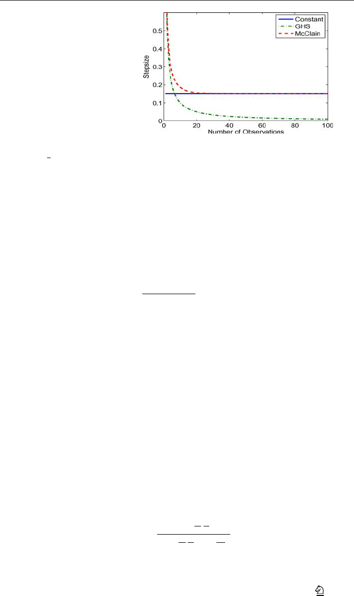
Fig. 2 Comparison of

deterministic stepsizes

where η ∈ (

, 1). These stepsizes do not decline as fast as the 1/n rule and can aid in faster

learning when there is an initial transient phase. Even-Dar and Mansour (2004) derives the

convergence rates for polynomial stepsize rules in the contextof Q-learning for MarkovDeci-

sion Processes. The best experimental value of η is shown to be about 0.85. The convergence

rate is shown to be polynomial in 1/(1 − γ ), where γ is the discount factor.

McClain’s formula

McClain’s formula combines the advantages of 1/n and constant stepsize formulas.

⎧

⎨

⎩

, if n = 1

n−1

1 + α

n−1

− ¯α

, if n ≥ 2

(10)

The stepsizes generated by this model satisfy the following properties:

>α

n+1

> ¯α, if α

> ¯α, (11)

<α

n+1

< ¯α, if α

< ¯α, (12)

lim

n→∞

= ¯α (13)

As illustrated in Fig. 2, if the initial stepsize (α

) is larger than the target stepsize ( ¯α) then

McClain’s formula behaves like the 1/n rule for the early iterations and as the stepsizes

approach ¯α, it starts mimicking the constant stepsize formula. The non-zero stepsizes can

capture changes in the underlying signal that may occur in the later iterations.

“Search then converge” (STC) algorithm

Darken and Moody (1991) suggests a “search then converge” (STC) procedure for computing

the stepsizes, as given by the formula,

= α



1 +





1 +

+ N



(14)

This formula keeps the stepsize large in the early part of the experiment where n  N

(which deﬁnes the “search mode”). During the “converge mode”, when n  N , the formula

Springer

174 Mach Learn (2006) 65:167–198

decreases as c/n. A good choice of the parameters would move the search in the direction of

the true value quickly and then bring about convergence as soon as possible. The parameters

of this model can be adjusted according to whether the algorithm is required to search for

the neighborhood in which the optimal solution (or true value) lies or to converge quickly to

the right value.

A slightly more general form which can be reduced to most of the deterministic stepsize

rules discussed above is the formula,

= α



+ a





+ a +n

− 1



(15)

Setting a = 0, b = 1 and n

= 0 gives us the polynomial learning rates,whereas setting b = 0

would give us the generalized harmonic stepsize rule. The STC formula can be obtained by

setting a = c/α

, b = N and η = 1. Adjusting the triplet, (a, b,η), enables us to control the

rate at which the stepsize changes at different stages of the estimation process. Using η<1

slows down the rate of convergence, which can help with problems which exhibit long tailing

behavior. The selection of the parameters a and b for the case where η = 1 is discussed in

Spall (2003) (Sections 4.5.2 and 6.6).

The major drawback of deterministic stepsize rules is that there is usually one or more

parameters that need to be preset. The efﬁciency of such rules would be dependent on picking

the right valuefor those parameters. For problems where we need to estimate several thousand

different quantities, it is unlikely that all of them converge to their true values at the same

rate. This is commonly encountered in applications such as dynamic programming, where

the estimation of a value function is desired and the values converge at varying rates as shown

in Fig. 3.

In practice, the stepsize parameters might be set to some global values, which may not

give the required convergence for the individual value functions.

2.2. Stochastic stepsize rules

One way of overcoming the drawbacks of deterministic stepsize rules is to use stochastic or

adaptive stepsize formulas that react to the errors in the prediction with respect to the actual

Fig. 3 Different rates of convergence of value functions

Springer

Mach Learn (2006) 65:167–198 175

observations. We let ˆε

−

n−1

, denote the observed error in the prediction at iteration

n. Most of the adaptive methods compute the stepsize as a function of these observed errors.

Kesten’s rule

Kesten (1958) proposes the following stochastic stepsize rule:

= α



b + K



(16)

where a, b and α

are positive constants to be calibrated. K

is the tracking signal at iteration

n which records the number of times that the error has changed signs. K

is recursively

computed as follows:



n, if n = 1, 2

n−1

+ 1

{ˆε

ˆε

n−1

<0}

, n > 2

(17)

where 1

{X}



1, if X is true

0, otherwise

This rule decreases the stepsize if the inner product of successive errors is negative and

leaves it unchanged otherwise. The idea is that if the successive errors are of the same sign,

the algorithm has not yet reached the optimal or true value and the stepsize needs to be kept

high so that this point can be reached faster. If the successive errors are of opposite signs, it is

possible that it could be due to random ﬂuctuation around the mean and hence, the stepsize

has to be reduced for stability and eventual convergence.

Mirozahmedov’s rule

Mirozahmedov and Uryasev (1983) formulates an adaptive stepsize rule that increases or

decreases the stepsize in response to whether the inner product of the successive errors is

positive or negative, along similar lines as in Kesten’s rule.

= α

n−1

exp[(aˆε

ˆε

n−1

− δ)α

n−1

] (18)

where a and δ are some ﬁxed constants. A variation of this rule, where δ is zero, is proposed

by Ruszczy´nski and Syski (1986). Both these rules bear resemblances to the class of expo-

nentiated gradient methods, where additive updating is performed on the logarithm of the

estimate (see Kivinen & Warmuth (1997) & Precup & Sutton (1997)).

Gaivoronski’s rule

Gaivoronski (1988) proposes an adaptive stepsize rule where the stepsize is computed as a

function of the ratio of the progress to the path of the algorithm. The progress is measured

in terms of the difference in the values of the smoothed estimate between a certain number

of iterations. The path is measured as the sum of absolute values of the differences between

Springer

176 Mach Learn (2006) 65:167–198

successive estimates for the same number of iterations.



n−1

if 

n−1

≤ γ

n−1

otherwise

(19)

where,



n−k

−



n−1

i=n−k

−

i+1

(20)

and γ

are pre-determined constants, and

denotes the estimate at iteration n.

Trigg’s rule

Trigg (1964) develops a tracking signal, T

, in order to monitor the forecasting process.

(21)

where,

= The smoothed sum of observed errors

(

1 − α

)

n−1

+ α ˆε

(22)

= The mean absolute deviation

(

1 − α

)

n−1

+ α|ˆε

| (23)

This value lies in the interval [−1, 1]. A tracking signal near zero would indicate that the

forecasting model is of good quality, while the extreme values would suggest that the model

parameters need to be reset. Trigg and Leach (1967) proposes using the absolute value of

this tracking signal as an adaptive stepsize.

trigg

=|T

| (24)

Trigg’s formula has the disadvantage that it reacts too quickly to short sequences of errors

with the same sign. A simple way of overcoming this, known as Godfrey’s rule (Godfrey,

1996) uses Trigg’s stepsize as the target stepsize in McClain’s formula. Another use of Trigg’s

formula is a variant known as Belgacem’s rule (Bouzaiene-Ayari, 1998) where the stepsize

is given by 1/K

. K

= K

n−1

+ 1ifα

trigg

< ¯α and K

= 1, otherwise, for an appropriately

chosen value of ¯α.

Chow’s method

Yet another class of stochastic methods uses a family of deterministic stepsizes and at each

iteration, picks the one that tracks the lowest error. Chow (1965) suggests a method where

three sequences of forecasts are computed simultaneously with stepsizes set to high, normal

and low levels (say, α +0.05, α and α − 0.05). If the forecast errors after a few iterations

Springer

Mach Learn (2006) 65:167–198 177

are found to be lower for either of the “high” or “low” level stepsizes, α is reset to that value

and the procedure is repeated.

Stochastic gradient adaptive (SGA) stepsize methods

Algorithms where the stepsizes are updated using stochastic gradient techniques are employed

in neural networks and signal processing applications. These methods attempt to optimize

the stepsize parameters in an on-line fashion, based on the instantaneous prediction errors,

so that they eventually converge to an ideal stepsize value. We consider a stochastic gradient

adaptive stepsize algorithm proposed by Benveniste, Metivier and Priouret (1990), where the

objective is to track a time-varying parameter, θ

, using noisy observations. In our context,

the observations would be modeled as

= θ

+ ε

, where ε

is a zero mean noise term.

The proposed method uses a stochastic gradient approach to compute stepsizes that minimize

E[(ˆε

)

], the expected value of the squared prediction error (which is as deﬁned earlier in

this section). The stepsize is recursively computed using the following steps:

= [α

n−1

+ μψ

n−1

ˆε

]

−

(25)

= (1 − α

)ψ

n−1

+ ˆε

(26)

where α

and α

−

are truncation levels for the stepsizes (α

−

≤ α

). Proper behavior of

this approximation procedure depends, to a large extent, on the value that is chosen for α

μ is a parameter that scales the product ψ

n−1

ˆε

, which has units of squared errors, to lie in

the suitable range for α. The ideal value of μ is problem speciﬁc and requires some tuning

for each problem.

Kalman ﬁlter

This technique is widely used in stochastic control where system states are sequentially

estimated as a weighted sum of old estimates and new observations (Stengel (1994), Section

4.3). The new state of the system θ

is related to the previous state according to the equation

= θ

n−1

+ w

, where w

is a zero mean random process noise with variance ρ

+ ε

denotes noisy measurements of the system state, where ε

is assumed to be white

gaussian noise with variance σ

. The Kalman ﬁlter provides a method of computing the

stepsize or ﬁlter gain (as it is known in this ﬁeld) that minimizes the expected value of the

squared prediction error and facilitates the estimation of the new state according to Eq. (5).

The procedure involves the following steps:

n−1

+ σ

= (1 − α

n−1

+ ρ

The Kalman ﬁlter gain, α

, adjusts the weights adaptively depending on the relative amounts

of measurement noise and the process noise. The implicit assumption is that the noise prop-

erties are known.

3. Optimal stepsizes for nonstationary data

In the presence of nonstationarity, the 1/n stepsize formula ceases to be optimal, since it

fails to take into account the biases in the estimates that may arise as a result of a trend in

the data. We derive a formula to compute the optimal stepsizes in terms of the noise variance

Springer

178 Mach Learn (2006) 65:167–198

and the bias in the estimates, in Section 3.1. We make note that we are using the principle of

certainty-equivalence, where we ﬁrst obtain an analytical expression for the optimal stepsizes

by replacing all random quantities with their expected values. We present, in Section 3.2, an

algorithm that computes approximations of the optimal stepsizes by using estimates of the

various unknown parameters. In Section 3.3, we provide our adaptation of the Kalman ﬁlter

for the nonstationary estimation problem.

3.1. An optimal stepsize formula

Weconsider abounded deterministic sequence {θ

}that variesslowlyover time. Our objective

is to form estimates of θ

using a sequence of noisy observations of the form

= θ

+ ε

where the ε

are zero-mean random variables that are independent and identically distributed

with ﬁnite variance σ

The smoothed estimate is obtained using the recursion deﬁned in Eq. (5) where α

denotes

the smoothing stepsize at iteration n.

Our problem becomes one of ﬁnding the stepsize that will minimize the expected error of

the smoothed estimate,

, with respect to the deterministic value, θ

. We denote the objective

function as, J(α

) = E[(

(α

) − θ

)

]. We wish to ﬁnd α

∈ [0, 1] that minimizes J (α

The observation at iteration n is unbiased with respect to θ

, that is, E[

] = θ

.We

deﬁne the bias in the smoothed estimate from the previous iteration as β

= E



−

n−1



− E



n−1



. The following proposition provides a formula for the variance of

n−1

Proposition 1. The variance of the smoothed estimate satisﬁes the equation:

Var [

] = λ

n = 1, 2,... (27)

where



(α

)

n = 1

(α

)

+ (1 −α

)

n−1

n > 1

(28)

Proof: We start by taking variances on both sides of Eq. (5)

Var[

] = (1 − α

)

Var[

n−1

] + (α

)

Var[

]

= (1 − α

)

Var[

n−1

] + (α

)

(29)

Since the initial estimate,

, is deterministic, Var[

] = (1 − α

)

Var[

] +

(α

)

Var[

] = (α

)

. For general n, it follows that,

Var[

] =



i=1

(α

)



j=i+1

(1 − α

)

We let λ



i=1

(α

)



j=i+1

(1 − α

)

. Substituting this in Eq. (29) gives us the recursive

expression in Eq. (28).

Wasan (1969) (pp. 27–28) derives a similar expression for the variance of an estimate

computed using the Robbins-Monro method for the special case where the stepsizes are of

the form α

= c/nb and the individual observations are uncorrelated with variance σ



Springer

Mach Learn (2006) 65:167–198 179

We propose the following theorem for solving the optimization problem.

Theorem 3. Given an initial stepsize, α

, and a deterministic initial estimate,

, the optimal

stepsizes that minimize the objective function can be computed using the expression,

(α

)

∗

= 1 −

(1 + λ

n−1

)σ

+ (β

)

n = 2, 3,... (30)

where β

denotes the bias (β

= θ

− E[

n−1

]) and λ

n−1

is deﬁned by the recursive expres-

sion in Eq. (28).

Proof: We can simplify the objective function as follows:

J(α

) = E[(

(α

) − θ

)

]

= E[((1 − α

)

n−1

+ α

− θ

)

]

= E[((1 − α

)(

n−1

− θ

) + α

(

− θ

))

]

= (1 − α

)

E[(

n−1

− θ

)

] + (α

)

E[(

− θ

)

]

+2α

(1 − α

)E[(

n−1

− θ

)(

− θ

)] (31)

Under our assumption that the errors ε

are uncorrelated, we have,

E[(

n−1

− θ

)(

− θ

)] = E[(

n−1

− θ

)]E[(

− θ

)]

= E[(

n−1

− θ

)] · 0

= 0

The objective function reduces to the following form:

J(α

) = (1 − α

)

E[(θ

−

n−1

)

] + (α

)

E[(

− θ

)

] (32)

In order to ﬁnd the optimal stepsize, (α

)

∗

, that minimizes this function, we obtain the ﬁrst

order optimality condition by setting

∂ J (α

)

∂α

= 0, which gives us,

−(1 − (α

)

∗

)E[(θ

−

n−1

)

] + (α

)

∗

E[(

− θ

)

] = 0 (33)

Solving this for (α

)

∗

gives us the following result,

(α

)

∗

E[(θ

−

n−1

)

]

E[(θ

−

n−1

)

] + E[(

− θ

)

]

(34)

The mean squared error term, E[(θ

−

n−1

)

], can be computed using the well known

bias-variance decomposition (see (Hastie, Tibshirani, & Friedman, 2001)), according to

which E[(θ

−

n−1

)

] = Var [

n−1

] + (β

)

. Using Proposition 1, the variance of

n−1

is ob-

tained as Var[

n−1

] = λ

n−1

. Finally, E[(

− θ

)

] = E[(ε

)

] = σ

, which completes

the proof.



Springer

180 Mach Learn (2006) 65:167–198

We state the following corollaries of Theorem 3 for special cases on the observed data

with the aim of further validating the result that we obtained for the general case where the

data is nonstationary.

Corollary 1. For a sequence with a static mean, the optimal stepsizes are given by,

(α

)

∗

∀ n = 1, 2,... (35)

given that the initial stepsize, (α

)

∗

= 1.

Proof: For this case, the mean of the observations is static (θ

= θ,n = 1, 2,...). The bias in

the estimate,

n−1

can be computed (see Wasan (1969), p. 27–28) as β



n−1

i=1



1 − α



where β

denotes the initial bias (β

= θ −

). Given the initial condition, (α

)

∗

= 1, we

have

, which would cause all further bias terms to be zero, that is, β

= 0 for

n = 2, 3,.... Substituting this result in Eq. (30) gives us,

(α

)

∗

n−1

1 + λ

n−1

(36)

We now resort to a proof by induction for the hypothesis that (α

)

∗

= 1/n and λ

= 1/n for

n = 1, 2,.... By deﬁnition, the hypothesis holds for n = 1, that is, λ

= ((α

)

∗

)

= 1. For

n = 2, we have (α

)

∗

= 1/(1 + 1) = 1/2. Also, λ

= (1 − 1/2)

(1) + (1/2)

= 1/2.

Now, we assume the truth of the hypothesis for n = m, that is, (α

)

∗

= λ

= 1/m.A

simple substitution of these results in Eqs. (36) and (28) gives us (α

m+1

)

∗

= λ

m+1

= 1/(m +

1). Thus, the hypothesis is shown to be true for n = m + 1. Hence, by induction, the result

is true for n = 1, 2,....



We note that our theorem for the nonstationary case reduces to the result for the stationary

case (Eq. (7)) which we had determined through variance minimization.

Corollary 2. For a sequence with zero noise, the optimal stepsizes are given by,

(α

)

∗

= 1 n = 1, 2,... (37)

Proof: For a noiseless sequence, σ

= 0. Substituting this in Eq. (30) gives us the desired

result.



3.2. The algorithmic procedure

In a realistic setting, the parameters of the series of observations are unknown. We propose

using the plug-in principle (see Bickel & Doksum (2001), pp. 104–105), where we form

estimates of the unknown parameters and plug these into the expression for the optimal

stepsizes. We assume that the sequence {θ

} varies slowly compared to the {ε

} process.

The bias is approximated by smoothing on the prediction errors according to the formula,

= (1 − ν

)

n−1

+ ν

(

−

n−1

), where ν

is a suitably chosen deterministic stepsize

rule. The idea is that averaging the current prediction error with the errors from the past

iterations will smooth out the variations due to noise to give us a reasonable approximation

Springer

Mach Learn (2006) 65:167–198 181

of the instantaneous bias. It is important to recognize that the estimate of the bias should be

updated on a faster time scale than the main algorithm (which means that a larger value of

should be used). At the same time, if ν

is too large, the result will be instability in the

estimate of the bias which can create its own problems. For this reason, we propose to ﬁnd

numerically using controlled experiments.

We ﬁrst deﬁne δ

= E[(

−

n−1

)

], the expected value of the squared prediction errors.

The following proposition provides a method to compute the variance in the observations.

Proposition 2. The noise variance, σ

, can be expressed as,

− (β

)

1 + λ

n−1

(38)

Proof: δ

can be written as,

= E[(

)

− 2

n−1

+ (

n−1

)

]

= E[(

)

] − 2E[

n−1

] + E[(

n−1

)

]

= Var [

] + (E[

])

− 2E[

n−1

]E[

] + Va r[

n−1

] + (E[

n−1

])

= σ

+ (θ

)

− 2E[

n−1

]θ

+ Va r[

n−1

] + (E[

n−1

])

= σ

+ λ

n−1

+ (θ

− E[

n−1

])

= (1 + λ

n−1

)σ

+ (β

)

(39)

Rearranging Eq. (39) gives us the desired result.



In order to estimate σ

, we approximate δ

by smoothing on the squared instanta-

neous errors. We use

to denote this approximation and compute it recursively:

(1 − ν

)

n−1

+ ν

(

−

n−1

)

. We justify this approximation using a similar line of rea-

soning as the one used for approximating the bias. The parameter λ

is approximated using

(

1 − α

)

n−1

(

)

. By plugging the approximations,

and

n−1

, into Eq. (39),

we obtain the following approximation of the noise variance:

(¯σ

)

− (

)

1 +

n−1

The optimal stepsize algorithm (OSA) which incorporates these steps is outlined in Fig. 4.

3.3. An adaptation of the Kalman ﬁlter

We note the similarity of OSA to the Kalman ﬁlter, where the gain depends on the relative

values of the measurement error and the process noise. We point out that in the applications

of the Kalman ﬁlter, the state is assumed to be stationary in the sense of expected value.

We present an adaptation of the Kalman ﬁlter for our problem setting where the parameter

evolves over time in a deterministic, nonstationary fashion. We later use this modiﬁed version

of the Kalman ﬁlter as a competing stepsize formula in our experimental comparisons.

Springer

182 Mach Learn (2006) 65:167–198

Fig. 4 The optimal stepsize algorithm

In our problem setting, the stochastic state increment (w

) from the original formulation

of the control problem, is replaced by a deterministic term which we simply deﬁne as w

− θ

n−1

. We replace the variance of w

by the approximation ( ¯ρ

)

= (

)

. We use the

same procedure as is used in OSA for computing the approximations, ( ¯σ

)

and ( ¯ρ

)

.We

incorporate these modiﬁcations to provide our adaptation of the Kalman ﬁlter, which involves

the following steps,

¯ρ

= (1 − ν

)¯ρ

n−1

+ ν

(

−

n−1

)

= (1 − ν

)

n−1

+ ν

(

−

n−1

)

(¯σ

)

− (¯ρ

)

1 +

n−1

+ (¯σ

)

= (1 − α

n−1

+ (¯ρ

)

Here, α

is our approximation of the Kalman ﬁlter gain and ν

is some appropriately chosen

deterministic stepsize series.

Alternative methods to estimate the variance (σ

) of the observation noise are described

in Jazwinski (1969) and later reviewed in DeFreitas, Niranjan and Gee (1998) and Penny and

Roberts (1998).

Springer

Mach Learn (2006) 65:167–198 183

4. Experimental results

In this section, we present numerical work comparing the optimal stepsize rule to other

stepsize formulas. Section 4.1 provides a discussion on the selection of parameters for the

stepsize rules, along with a sensitivity analysis for the parameters of OSA. We illustrate the

performance of OSA as compared to other stepsize rules using scalar functions in Section

4.2. The functions that we choose are similar to those encountered in dynamic programming

algorithms, typical examples of which are shown in Fig. 3. In this controlled setting, we

are able to adjust the relative amounts of noise and bias, and draw reasonable conclusions.

In the remaining sections, we compare the performance of the stepsize rules for estimating

value functions in approximate dynamic programming applications. Section 4.3 deals with a

batch replenishment problem where decisions are to be made over a ﬁnite horizon. In section

4.4, we consider a problem class we refer to as the “nomadic trucker”. This is an inﬁnite

horizon problem involving the management of a multiattribute resource, with similarities to

the well-known taxi problem.

4.1. Selection of parameters

In order to smooth the estimates of the parameters used in OSA, we used a McClain stepsize

rule. The McClain target stepsize is the sole tunable parameter in OSA. We performed a

variety of experiments with different choices of this target stepsize in the range of 0 to 0.2.

We compared the estimates against their true values and found that for target stepsizes in the

range 0.01 to 0.1, the ﬁnal estimates are not that different. The percentage errors from the

true values for different problems are illustrated in Table 1. We choose a target stepsize of

0.05 since it appears to be very robust in the sense mentioned above.

The parameter η for the polynomial learning rate is set to the numerically optimal (as

demonstrated in Even-Dar and Mansour (2004)) value of 0.85. The parameters for the STC

algorithm are chosen by optimizing over all the possible combinations of a and b from

among twenty different values each of a, varying over the range of 1–200, and b,over

the range of 0–2000. In the experiments to follow, we concern ourselves mainly with two

classes of functions—class I functions, which are concave and monotonically increasing,

and class II functions, which undergo a rapid increase after an initial stationary period and

are not concave. (a = 6, b = 0,η = 1) is found to work best for class I functions, whereas

(a = 12, b = 0,η = 1) produces the best results for class II functions. We choose a target

stepsize, ¯α = 0.1, for the McClain stepsize rule. The parameters for Kesten’s rule were set

to a = b = 10. We implement the adaptation of the Kalman ﬁlter with the same parameter

settings as for OSA.

Table 1 Choosing the parameter

¯ν for OSA: The entries denote

percentage errors from the true

values averaged over several

sample realizations

¯ν Scalar functions Batch replenishment Nomadic trucker

0.00 3.366 2.638 2.511

0.01 3.172 2.657 2.654

0.02 2.896 2.676 2.540

0.05 2.274 2.678 2.531

0.10 2.674 2.639 2.519

0.20 3.567 2.683 2.960

Springer

184 Mach Learn (2006) 65:167–198

In the implementation of the SGA stepsize algorithm, we set the lower truncation limit to

0.01. As pointed out in Kushner and Yin (1997), the upper truncation limit, α

seems to affect

the solution quality signiﬁcantly. Setting α

to a low value was seen to result in poor initial

estimates, especially for problems with low noise variance, while increasing α

, on the other

hand, produced poor estimates for problems with high noise. We set α

= 0.3, as suggested

in the same work, for all the problems that we consider. According to the cited article, for a

certain class of problems, the performance of the algorithm is fairly insensitive to the scaling

parameter, μ, if it is chosen in the range [0.0001,0.0100]. However, in our experiments,

the stepsizes were observed to simply bounce back and forth between the truncation limits

(α

and α

−

) for problems where the order of magnitude of the errors exceeded that of the

stepsizes, if μ was not chosen to be sufﬁciently small. Then again, too low a value of μ

caused the stepsizes to hover around the initial value. We concluded that the parameter μ is

problem speciﬁc and has to be tuned for different problem classes. We tested the algorithm

for μ ranging from 10

−9

to 0.2. It was inconclusive as to which value of μ worked best. There

did not seem to be a consistent pattern as to how the value of μ affected the performance

of the algorithm for different noise levels or function slopes. For the scalar functions and

the batch replenishment problem, we chose a value of μ (= 0.001) in the range suggested

in the cited article, as it seemed to work moderately well for those problem classes. For the

nomadic trucker problem, μ had to be set to 10

−6

for proper scaling.

4.2. Illustrations on scalar functions

For testing the proposed algorithm, we use it to form estimates or predictions for data series

that follow certain functional patterns. The noisy observations of the data series are generated

by adding a random error term to the function value corresponding to a particular iteration.

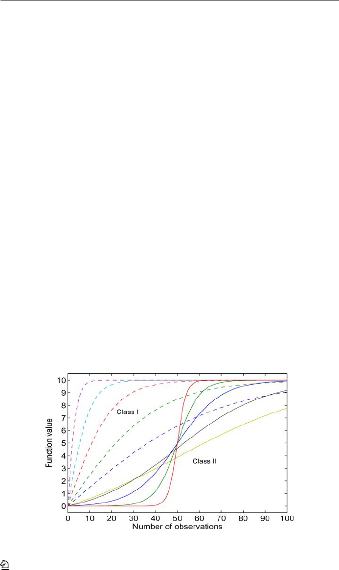
The function classes that we consider are shown in Fig. 5. The functions belonging to class

I are strictly concave. This class is probably the most common in dynamic programming.

Class II functions remain more or less constant initially, then increase more quickly before

stabilizing, with a sudden increase after 50 observations. Functions of this type arise when

there is delayed learning, where the algorithm has to go through a number of iterations before

undergoing signiﬁcant learning. This is encountered in problems such as playing a game,

Fig. 5 Two classes of functions, each characterized by the timing of the upward shift. Five variations were

used within each class by varying the slope

Springer

Mach Learn (2006) 65:167–198 185

Fig. 6 Observations made at three different levels of variance in the noise

Fig. 7 Sensitivity of stepsizes to variations in a class II function

where the outcome of a particular action is not known until the end of the game and it takes a

while before the algorithm starts to learn “good” moves. Each of these functions is measured

with some noise that has an assumed variance. In Fig. 6, we illustrate the noisy observations

at three different values of the noise variance.

The performance measure that we use for comparing the stepsize rules is the average

squared prediction error across several sample realizations over all the different functions

belonging to a particular class. Figure 7 illustrates stepsize values averaged over several

sample realizations of moderately noisy observations from a class II function. We compare

the stepsizes obtained using the various stepsize rules, both deterministic and stochastic. The

advantages of stochastic stepsizes are best illustrated for this function class. By the time the

function value starts to increase, the stepsize computed using any of the deterministic rules

would have dropped to such a small value that it would be unable to respond to changes in

the observed signal quickly enough. The stochastic stepsize rules are able to overcome this

problem. Even in the presence of moderate levels of noise, the SGA stepsize algorithm, the

Springer

186 Mach Learn (2006) 65:167–198

Fig. 8 Sensitivity of stepsizes to noise levels. The SGA stepsize algorithm is used with two parameter settings

to bring out the sensitivity of the procedure to the scaling parameter, μ: SGA(1) with μ = 0.001 and SGA(2)

with μ = 0.01

Kalman ﬁlter and OSA are seen to be able to capture the shift in the function and produce

stepsizes that are large enough to move the estimate in the right direction. We point out that

the response of the SGA stepsize algorithm is highly dependent on μ, which if set to small

values, could cause the stepsizes to be less responsive to shifts in the underlying function.

OSA, on the other hand, is much less sensitive to the target stepsize parameter, ¯ν.

An ideal stepsize rule should have the property that the stepsize should decline as the noise

level increases. Speciﬁcally, as the noise level increases, the stepsizes should decrease in order

to smooth out the error due to noise. The deterministic stepsize rules, being independent of

the observed data, would fail in this respect. In Fig. 8, we compare the average stepsizes

obtained using various adaptive stepsize rules for a class II function at different levels of

the noise variance. The high sensitivity of the SGA stepsize algorithm to the value of μ is

evident from this experiment. A higher value of μ causes the stepsizes to actually increase

with higher noise. Among the adaptive stepsize rules, only the Kalman ﬁlter and OSA seem

to demonstrate the property of declining stepsizes with increasing noise variance.

Table 2 compares the performance of the stepsize rules for concave, monotonically in-

creasing functions. Value functions encountered in approximate dynamic programming ap-

plications typically undergo this kind of growth across the iterations. n refers to the number of

observations, the entries in each cell denote the average mean squared error in the estimates

and the ﬁgures in italics represent the rank performance of the stepsize rule. The errors are

computed as the difference in the estimates from the instantaneous value of the function,

which in this case starts from a small initial value and rises steadily for several observations,

before settling on a stationary value. We are interested in how the stepsize rules contribute

to the rate at which the function is learnt.

The results indicate that in almost all the cases, OSA either produces the best results, or

comes in a close second or third. It performs the worst on the very high noise experiments

where the noise is so high that the data is effectively stationary. It is not surprising that a simple

deterministic rule works best here, but it is telling that the other stepsize rules, especially the

adaptive ones, have noticeably higher errors as well.

Springer

Mach Learn (2006) 65:167–198 187

Table 2 A comparison of stepsize rules for class I functions, which are concave and monotonically

increasing

Noise n 1/n 1/n

STC McClain Kesten SGA Kalman OSA

= 1 25 5.697 2.988 0.483 1.747 0.354 0.364 0.365 0.304

rank 8 7 5 6 2 3 4 1

50 5.690 2.369 0.313 0.493 0.196 0.202 0.206 0.146

rank 8 7 5 6 2 3 4 1

75 4.989 1.711 0.198 0.167 0.130 0.172 0.144 0.098

rank 8 7 6 4 2 5 3 1

= 10 25 6.101 3.440 1.560 2.323 2.643 1.711 2.177 1.481

rank 8 7 2 5 6 3 4 1

50 5.893 2.609 0.891 0.991 1.590 1.213 1.306 0.908

rank 8 7 1 3 6 4 5 2

75 5.127 1.878 0.584 0.649 1.130 0.888 0.945 0.774

rank 8 7 1 2 6 4 5 3

= 100 25 10.014 8.052 13.101 8.408 26.704 17.697 12.272 10.263

rank 3 1 6 2 8 7 5 4

50 7.871 4.936 6.520 5.823 15.163 16.405 7.927 7.412

rank 5 1 3 2 7 8 6 4

75 6.434 3.465 4.444 5.434 10.863 16.223 6.060 7.231

rank 5 1 2 3 7 8 4 6

Table 3 A comparison of stepsize rules for class II functions (which undergo delayed learning).

Noise n 1/n 1/n

STC McClain Kesten SGA Kalman OSA

= 1 25 0.418 0.298 0.222 0.229 0.279 0.209 0.220 0.183

rank 8 7 4 5 6 2 3 1

50 13.457 10.715 3.704 6.221 2.670 2.459 4.925 2.737

rank 8 7 4 6 2 1 5 3

75 30.420 15.817 0.469 1.187 0.257 0.239 0.271 0.205

rank 8 7 5 6 3 2 4 1

= 10 25 0.796 0.724 1.967 0.784 2.608 1.356 1.040 0.962

rank 3 1 7 2 8 6 5 4

50 13.674 11.008 4.713 6.781 4.147 5.090 7.131 5.753

rank 8 7 2 5 1 3 6 4

75 30.556 15.983 1.107 1.643 1.260 1.406 1.523 1.079

rank 8 7 2 6 3 4 5 1

= 100 25 4.552 4.941 19.393 6.268 26.023 16.568 8.829 8.490

rank 1 2 7 3 8 6 5 4

50 15.292 13.039 13.998 11.402 17.763 19.299 12.435 12.829

rank 6 4 5 1 7 8 2 3

75 31.544 17.431 7.706 6.468 11.224 16.633 8.560 8.299

rank 8 7 2 1 5 6 4 3

Table 3 compares the stepsize rules for functions which remain constant initially, then

undergo an increase in their value (the maximum rate of increase occurs after about 50

iterations) before converging to a stationary value. We notice that, for all the stepsize rules,

the errors are very small to begin with as a result of the initial stationary phase of the function.

As the transient phase sets in after about 50 observations, the errors show a dramatic increase.

Springer

188 Mach Learn (2006) 65:167–198

In the ﬁnal stationary phase of the function, the errors drop back to smaller values (for most

of the stepsize rules). Here again, OSA is seen to work well for moderate levels of noise, and

even otherwise, it performs comparably well.

To summarize, OSA is found to be a competitive technique, irrespective of the problem

class and the sample size as long as the noise variance is not too high.

4.3. Finite horizon problems: Batch replenishment

Dynamic programming techniques are used to solve problems where decisions have to be

made using information that evolves over time. The decisions are chosen so as to optimize

the expected value of current rewards plus future value.

For our experiments, we formulated the optimality equations around the post-decision

state variable (designated R

), which is the state immediately after a decision is made. We

let C(R

t−1

, W

, x

) be the reward obtained by taking action x

∈ X

when in state R

t−1

and

the exogenous information is W

. The resulting state R

is a function of R

t−1

, W

and x

The value associated with each state can be computed using Bellman’s optimality equations.

When constructed around the post-decision state variable, R

t−1

, the optimality equations take

on the following form:

t−1

) = E



max

∈X

[C(R

t−1

, W

, x

) + γ V

)]|R

t−1



∀t = 1, 2,...,T (40)

The values thus computed deﬁne an optimal policy, which enables us to determine the best

action, given a particular state.

When the number of possible states is large, computation of values using sweeps over the

entire state space can become intractable. In order to overcome this problem, approximate

dynamicprogrammingalgorithmshavebeen developedwhich step forward in time, iteratively

updating the valuesof only those states that are actually visited. If each state is visitedinﬁnitely

often, then the estimates of the values of individual states, as computed by the forward

dynamic programming algorithm, converge to their true values (Bertsekas & Tsitsiklis, 1996).

However, each iteration could be computationally expensive and we face the challenge of

obtaining reliable estimates of the values of individual states in a few iterations, which is

required to determine the optimal policy.

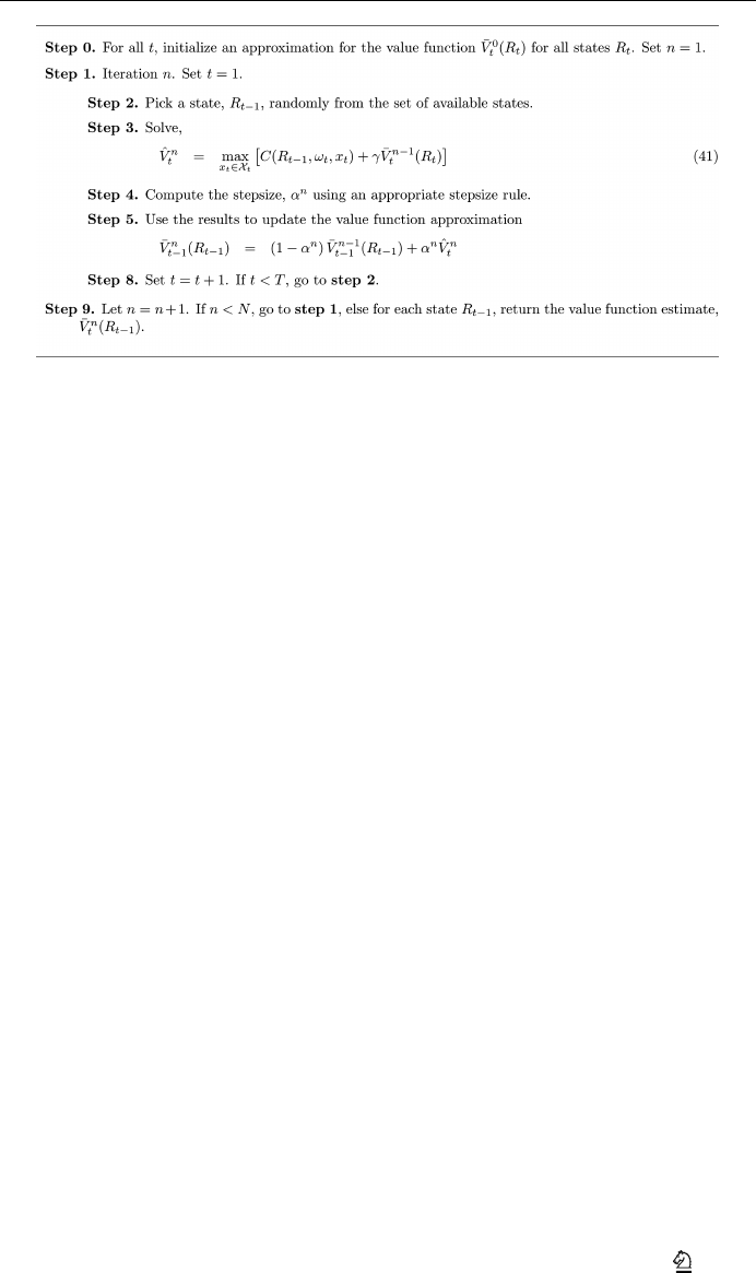
Figure 9 outlines a forward dynamic programming algorithm for ﬁnite horizon problems,

where we step forward in time, using an approximation of the value function from the pre-

vious iteration. We solve the problem for time t, where we randomly sample the exogenous

information at time t (Eq. (41). Here, ω

denotes a sample realization of the random infor-

mation at time t. We then use the results to update the value function for time t − 1 in Eq.

(42), which is an approximation of the expectation in Eq. (40).

We now consider the batch replenishment problem, where orders have to be placed for a

product at regular periods in time over a planning horizon to satisfy random demands that

may arise during each time period. The purchase cost is linear in the number of units of

product ordered. Revenue is earned by satisfying the demand for the product that arises in

each time period. The objective is to compute the optimal order quantity for each resource

state in any given time period.

The problem can be set up as follows. We ﬁrst deﬁne the following terms,

T = The time horizon over which decisions are to be made

γ = The discount factor

c = The order cost per unit product ordered

Springer

Mach Learn (2006) 65:167–198 189

Fig. 9 A generic forward dynamic programming algorithm

p = The payment per unit product sold

= The random demand for the product in time period t

= The amount of resource available at the end of time period t

= The quantity ordered in time period t

The contribution, C(R

t−1

, x

), obtained by ordering amount x

, when there are R

t−1

units of resource available and the demand for the next time period is

is obtained as,

C(R

t−1

, x

) = p[min(R

t−1

)] − cx

The new state is computed using the transition equation, R

= [R

t−1

−

]

+ x

. The ob-

jective is to maximize the total contribution from all the time periods, given a particular

starting state. The optimal order quantity at any time period maximizes the expected value of

the sum of the current contribution and future value. We may also set limits on the maximum

amount of resource (R

max

) that can be stored in the inventory and the maximum amount of

product (x

max

) that can be ordered in any time period.

We use the forward dynamic programming algorithm in Fig. 9, with the optimal stepsize

algorithm embedded in step 4, toestimatethe valueof eachresourcestate, R = 0, 1,...,R

max

for each time period, t = 1, 2,...,T − 1. We start with some initial estimate of the value

for each state at each time period. Starting from time t = 1, we step forward in time and

observe the value of each resource state that is visited. After a complete sweep of all the time

periods, we update the estimates of the values of all the resource states that were visited,

using a stochastic gradient algorithm. This is done iteratively until some stopping criterion

is met. We note that there may be several resource states that are not visited in each iteration.

We compare OSA against other stepsize rules—1/n,1/n

, STC, Kalman ﬁlter and SGA

stepsize algorithm, in its ability to estimate the value functions for the problem. The size of

the state space is not too large, which enables us to compute the optimal values of the resource

states using a backward dynamic programming algorithm. We consider two instances of the

batch replenishment problem—instance I, where a demand occurs every time period and

instance II, where the demand occurs only during the last time period. Table 4 lists the values

of the various parameters used in the two problem instances. In both cases, there are 26

resource states and 20 time periods, which gives us over 500 individual values that need to

be estimated.

Springer

190 Mach Learn (2006) 65:167–198

Table 4 Parameters for the

batch replenishment problem

Parameter Instance I Instance II

Demand Range [4, 5] [20, 25]

max

25 25

max

T 20 20

c 22

p 55

Table 5 Percentage error in the estimates from the optimal values, averaged over all the resource states

at all the time periods, as a function of the average number of observations per state. The ﬁgures in italics

denote the standard deviations of the values to the left.

Instance I - Regular Demands

γ n 1/n 1/n

STC SGA Kalman OSA

0.8 10 12.18 0.02 9.84 0.02 3.63 0.02 8.63 0.02 2.88 0.02 2.71 0.02

20 8.77 0.01 6.27 0.01 1.44 0.01 2.78 0.01 1.60 0.01 1.29 0.01

40 6.80 0.01 4.23 0.01 0.90 0.00 1.14 0.00 1.06 0.00 0.97 0.00

60 5.94 0.01 3.35 0.01 0.73 0.00 1.16 0.00 0.78 0.00 0.91 0.00

0.9 10 17.70 0.02 14.45 0.02 4.73 0.02 12.88 0.02 3.24 0.02 2.77 0.02

20 13.23 0.02 9.67 0.02 1.81 0.01 4.18 0.01 2.72 0.01 1.84 0.01

40 10.50 0.02 6.81 0.01 1.36 0.00 1.37 0.00 2.14 0.00 1.77 0.00

60 9.31 0.02 5.54 0.01 1.27 0.00 1.74 0.00 1.64 0.00 1.71 0.00

0.95 10 21.68 0.03 17.72 0.02 5.26

0.02 15.84 0.02 4.05 0.02 3.11 0.02

20 16.39 0.02 11.91 0.02 2.24 0.01 4.89 0.01 3.91 0.01 2.80 0.01

40 13.00 0.02 8.27 0.02 2.11 0.00 1.92 0.00 3.25 0.00 2.76 0.01

60 11.50 0.02 6.68 0.02 2.05 0.00 2.52 0.00 2.64 0.00 2.65 0.01

Instance II - Lagged Demands

γ n 1/n 1/n

STC SGA Kalman OSA

0.8 10 31.61 0.03 27.72 0.03 14.86 0.02 25.66 0.02 19.29 0.03 12.38 0.02

20 26.65 0.02 21.74 0.02 7.98 0.01 13.21 0.01 8.81 0.02 4.67 0.01

40 22.77 0.02 16.89 0.02 3.57 0.00 3.70 0.00 1.86 0.01 0.74 0.00

60 20.82 0.02 14.41 0.01 2.02 0.00 0.95 0.00 0.34 0.00 0.36 0.00

0.9 10 50.34 0.03 46.00 0.03 29.03 0.03 43.64 0.03 37.23 0.03 24.50 0.03

20 44.86 0.03 38.96 0.03 17.17 0.02 27.04 0.02 20.22 0.03 8.72 0.02

40 40.34 0.03 32.77 0.02 8.35 0.02 8.53 0.02 3.91 0.02 1.29 0.01

60 37.98 0.03 29.35 0.02 4.86 0.01 1.86 0.01 0.64 0.02 0.66 0.00

0.95 10 62.94 0.02 58.87 0.02 40.14

0.03 56.60 0.03 50.63 0.03 33.65 0.03

20 57.79 0.03 51.85 0.03 24.09 0.03 38.04 0.03 29.07 0.04 10.59 0.03

40 53.34 0.03 45.21 0.03 11.58 0.03 11.75 0.03 5.53 0.04 1.61 0.02

60 50.92 0.03 41.34 0.03 6.72 0.02 2.33 0.02 1.19 0.03 1.09 0.01

In Table 5, we compare the various stepsize rules based on the percentage errors in the

value function estimates with respect to the optimal values. n denotes the average number of

observations per resource state. The entries in the table denote averages across all the resource

states and time periods. The inability of simple averaging (the 1/n rule) to produce good

estimates for this class of problems is clearly demonstrated for this instance. Compared to the

Springer

Mach Learn (2006) 65:167–198 191

Fig. 10 Percentage errors in the value estimates with respect to the true values for an instance of the batch

replenishment problem

other deterministic rules, the STC rule is seen to work much better most of the time, almost

on par with the adaptive stepsize rules. Experiments in this problem class demonstrates the

improvement that can be brought about in the estimates by using an adaptive stepsize logic,

especially in the initial transient period. In almost all the cases, OSA is seen to outperform

all the other methods. Figure 10 gives a better illustration of the relative performance of the

stepsize rules. Here, we compare the percentage errors as a function of the average number

of observations per resource state. OSA is clearly seen to work well, giving much smaller

error values than the remaining rules even with very few observations.

4.4. Inﬁnite horizon problems: The nomadic trucker

We use an inﬁnite horizon forward dynamic programming algorithm (see Fig. 11) to estimate

value functions for a grid problem, namely, the nomadic trucker, which is similar to the well-

known taxicab problem. In the nomadic trucker problem, the state (R) of the trucker at any

instant is characterized by several attributes such as the location, trailer type and day of week.

When in a particular state, the trucker is faced with a random set of decisions, X(ω), which

could include decisions to move a load and decisions to move empty to certain locations.

The trucker may “move empty” to his current location, which represents a decision to do

Fig. 11 A basic approximate dynamic programming algorithm for inﬁnite horizon problems

Springer

192 Mach Learn (2006) 65:167–198

Table 6 Percentage error in the estimates from the optimal values, averaged over all the resource states,

as a function of the average number of observations per state. The ﬁgures in italics denote the standard

deviations of the values to the left

γ n 1/n 1/n

STC SGA Kalman OSA

0.80 5 27.37 0.18 24.96 0.19 17.24 0.21 27.28 0.17 19.78 0.18 15.35 0.21

10 18.17 0.14 14.56 0.13 5.62 0.08 12.36 0.11 5.60 0.08 4.86 0.07

15 14.78 0.12 10.81 0.11 3.51 0.05 6.25 0.06 3.67 0.04 3.19 0.05

20 12.81 0.11 8.70 0.09 2.85 0.04 3.86 0.04 3.10 0.04 2.57 0.04

0.90 5 44.67 0.17 41.76 0.18 29.55 0.21 44.53 0.17 30.80 0.19 23.77 0.23

10 35.70 0.16 31.02 0.16 13.85 0.13 27.77 0.14 9.46 0.12 8.77 0.13

15 31.78 0.14 26.20 0.13 8.53 0.09 17.74 0.10 4.23 0.08 4.83 0.08

20 29.32 0.13 23.17 0.12 5.94 0.07 11.36 0.07 2.68 0.04 3.18 0.06

0.95 5 63.27 0.14 60.66 0.15 47.48

0.18 63.23 0.14 46.50 0.21 36.61 0.23

10 55.99 0.14 51.53 0.14 30.91 0.14 48.44 0.13 19.79 0.15 17.96 0.15

15 52.51 0.13 46.94 0.13 23.61 0.11 37.54 0.12 10.67 0.10 11.40 0.11

20 50.24 0.12 43.87 0.12 19.32 0.08 29.17 0.09 6.61 0.08 8.05 0.09

nothing. His choice is determined by the immediate rewards obtained by taking a particular

course of action as well as the discounted value of the future state as represented in Eq. (42).

(R,ω

, x) denotes a transformation function indicating the new resource state when

resource R is acted upon by decision x, given a sample realization (ω

) of the random

exogenous information.

The size of the state space that we consider is 840 (40 locations, 3 trailer types and 7 days

of week), which makes the problem rich enough for the approximate dynamic programming

techniques to be interesting. At the same time, computation of the optimal values analytically

using backward dynamic programming is tractable. We point out that the states at each

iteration are picked at random, that is, we follow an “exploration” policy. We compare various

stepsize rules for estimating the values associated with the resource states for discount factors

of 0.8, 0.9 and 0.95.

Table 6 illustrates the performance of the competing stepsize rules for different values of

the discount factor. The entries correspond to the average errors (along with their standard

deviations) in the value estimates over several samples, as a percentage of the optimal values

of the states. OSA is found to work well, outperforming the remaining methods most of the

time. Compared to the other methods, STC is seen to work fairly well for this problem class

whereas the SGA stepsize algorithm (with parameter settings, μ = 10

−6

and α

= 0.3),

works poorly. The modiﬁed version of the Kalman ﬁlter is also found to work well in this

setting, especially towards the later part of the experiment. A better picture of the relative

performance of the various stepsize rules can be obtained from Fig. 12, which shows the

progress of the percentage errors in the value estimates with increasing number of observa-

tions. The gains provided by OSA over the other stepsize rules, especially with fairly small

number of observations, are clearly evident from this graph.

4.5. Analysis

In this section, we address two questions to help provide insights into the behavior of the

OSA algorithm. First, we try to provide additional support for why the algorithm works well.

Second, we investigate the behavior of the algorithm when applied to purely stationary data.

The primary argument supporting the strong performance of the algorithm is that the

stepsizes produced are optimal (in terms of minimizing the expected mean squared error)

Springer

Mach Learn (2006) 65:167–198 193

Fig. 12 Percentage errors in the value estimates with respect to the true values for an instance of the nomadic

trucker problem

if the bias and variance are known. Since these parameters have to be estimated in most

settings, the issue boils down to how well we are able to estimate these quantities. We

proceed to provide some evidence supporting the claim that we do a reasonably good job of

estimating these parameters.

Our analysis makes use of the scalar functions described in Section 4.2. We computed the

estimates of the standard deviation (σ ) of the noise and the bias (β) for σ = 1 and σ = 100.

The results are tabulated in Fig. 13, which illustrates the evolution of the estimates of the bias

Fig. 13 Estimate of the standard deviation and bias for low noise (σ = 1) and high noise (σ = 100) using

OSA for 20 sample realizations

Springer

194 Mach Learn (2006) 65:167–198

Fig. 14 Empirical convergence of OSA for different values of σ, with stationary observations

and the standard deviation using OSA for a class I function for 20 sample realizations. The

relative biases were computed by taking the difference between the absolute values of the

estimated bias and the true bias, and scaling it with respect to σ . The estimate of σ appears to

be unbiased and relatively accurate for both the low and high noise cases, with the exception

of the ﬁrst few iterations. The difference between the actual and estimated bias was typically

within ±σ/2 (with even more accurate results for the high noise case). We show an average

(indicated by the thick green line) across all the sample realizations, which suggests that our

estimates are unbiased.

We repeated the experiments for class II functions and were able to obtain very similar

results. In all the cases that we considered, we were able to obtain estimates of bias and

standard deviation that lay well within ≈±σ/2. The good performance of OSA for different

problem classes can be attributed to its ability to produce reasonably accurate estimates of

the bias and the standard deviation.

We now analyze the behavior of OSA in a stationary environment. OSA was designed for

the general case where the process could be nonstationary. It would be desirable to establish

the convergence of the algorithm when the observations arise from a stationary series. For

this case, we may use a target stepsize of zero for updating the parameters of average errors

(

) and squared errors (

). This would be equivalent to using a 1/n rule for updating these

parameters.

It is well known that a stepsize sequence will converge if it satisﬁes

1/n ≤ α

≤ c/n for n = 1, 2,... (43)

where c is some appropriately chosen positive constant. A proof that OSA satisﬁes α

≥ 1/n

is provided in Appendix A. We believe the second inequality is also true, but as of this writing

we have not been able to prove it. As an alternative, we offer some experimental evidence

to support the conjecture. We generated a thousand different sample sequences of stepsizes

using OSA for σ = 1 and σ = 100. The stepsize sequences are shown in ﬁg. 14 which shows

that the stepsizes fall within the range 1/n ≤ α

≤ 10/n. The lower bound is guaranteed.

We have not been able to ﬁnd an instance, for any variance or error distribution (we also

conducted runs assuming both uniform and normal distributions for the errors), where the

upper bound is violated.

5. Conclusions

We have introduced a new stepsize rule that minimizes the mean squared error in the presence

of transient data such as those that arise in approximate dynamic programming. The stepsizeis

Springer

Mach Learn (2006) 65:167–198 195

optimal for the parameters-known case (where we know the bias and variance). We propose a

method for estimating the bias and variance for the more realistic case where these parameters

are not known, and show, for three classes of adaptive estimation problems, that the new

formula works consistently well, and often better than the most popular formulas available

in the literature. Like the learning rate for the Kalman ﬁlter, our formula provides stepsizes

that approach 1 as the variance of the noise goes to zero, and approaches 1/n as the bias

approaches zero (as would occur with stationary data). Unlike the Kalman ﬁlter, our formula

is optimized for data coming from a series with a mean that is consistently rising or falling

over time.

We have tested the optimal stepsize algorithm for monotonically increasing concave func-

tions as well as functions where there is delayed learning. The optimal stepsize algorithm

is found to perform quite well in the presence of nonstationarity and give consistently good

results over the entire range of functions tested. The performance of our rule, as with all

stochastic stepsize rules, degrades somewhat in the presence of very high noise.

We have also applied the stepsize rules in the context of approximate dynamic program-

ming where we consider both ﬁnite and inﬁnite horizon problems. We employ OSA for

updating the value functions of resource states. Even though some of the assumptions that

we made regarding the nature of the observations, in particular that the observations are

independent and identically distributed, do not hold in the context of approximate dynamic

programming, OSA is still found to give much faster convergence to the optimal value as

compared to other stepsize rules for several different instances of the batch replenishment

and the nomadic trucker problems.

We conclude from our exercises that the optimal stepsize rule can give substantially better

results compared to a deterministic rule even with a fairly small number of observations and

it is also a superior alternative to most other adaptive stepsize rules in a variety of settings.

It requires a single parameter that has to be preset, namely the target stepsize parameter

for updating the estimates of bias, squared error and variance coefﬁcient. This parameter is

unitless, and does not have to be changed when the input data is scaled. We were also able

to identify a small range for this parameter over which the algorithm is found to be robust.

Finally, we point out that many of the deterministic stepsize rules, if properly tuned for

speciﬁc applications, can work better than adaptive rules such as OSA, especially if the noise

level is quite high. They also involve less computational overhead and a tradeoff has to be

made depending on the application considered. The value of OSA is that it is robust, and will

adjust to the behavior of individual parameters within a model.

Appendix

A. Partial proof of inequality (43)

We let K

= (

)

. From the deﬁnitions of

and

, it follows that 0 ≤ K

≤ 1. We

may now rewrite the expression for the stepsize by rearranging the major equations from the

algorithm described in Fig. 4:

n−1

+ K

n−1

+ 1

(44)

The ﬁrst of the inequalities in Eq. (43) can be proved using induction. We begin by assuming

= 1. By the deﬁnition of

, this implies that

= 1. For general n, we assume that

n−1

= 1/(n − 1) + L

n−1

(45)

Springer

196 Mach Learn (2006) 65:167–198

where 0 ≤ L

≤ 1.

We can write the stepsize as,

n−1

+ K

n−1

+ 1

n−1

+ L

n−1

+ K

n−1

+ L

n−1

+ 1

(n − 1)

n−1

+ n(n − 1)K

n(n −1)L

n−1

+ n

≥

This allows us to write,

= 1/n + M

(46)

where 0 ≤ M

≤ 1. Substituting Eqs. (45) and (46) into the deﬁnition of

from Section

3.2, we may write:



1 −

− M





n − 1

+ L

n−1





+ M



+ L

n−1



n − 1

− M









n−1

n − 1



≥

Thus, the following sequence of inequalities hold true for all n:

n−1

≥

n − 1

⇒ α

≥

⇒

≥

Acknowledgments The authors would like to acknowledge the helpful comments of James Spall, as well as

those of three anonymous referees who made several valuable suggestions that improved the presentation and

pointed out areas of the literature we had originally overlooked. This research was supported in part by grant

AFOSR-FA9550-05-1-0121 from the Air Force Ofﬁce of Scientiﬁc Research and NSF grant CMS-0324380.

References

Benveniste, A., Metivier, M., & Priouret, P. (1990). Adaptive algorithms and stochastic approximations,New

York: Springer-Verlag.

Bertsekas, D., & Tsitsiklis, J. (1996). Neuro-dynamic programming. Belmont, MA: Athena Scientiﬁc.

Bickel, P. J., & Doksum, K. A. (2001). Mathematical statistics—Basic ideas and selected topics volume 1.

Upper Saddle River, NJ: Prentice Hall.

Blum, J. (1954a). Approximation methods which converge with probability one. Annals of Mathematical

Statistics, 25, 382–386.

Springer

Mach Learn (2006) 65:167–198 197

Blum, J. (1954b). Multidimensional stochastic approximation methods. Annals of Mathematical Statistics,

25, 737–744.

Bouzaiene-Ayari, B. (1998). Private communication.

Bouzeghoub, M., Ellacott, S., Easdown, A., & Brown, M. (2000). On the identiﬁcation of non-stationary linear

processes. International Journal of Systems Science, 31(3), 273–286.

Brossier, J.-M. (1992). Egalization adaptive er estimateion de phase: Application aux Communications Sous-

Marines, PhD thesis, Institut National Polytechnique de Grenoble.

Brown, R. (1959). Statistical forecasting for inventory control. New York: McGraw-Hill.

Brown, R. (1963). Smoothing, forecasting and prediction of discrete time series, Englewood Cliffs, N.J.:

Prentice-Hall.

Chow, W. M. (1965). Adaptive control of the exponential smoothing constant. The Journal of Industrial

Engineering.

Darken, C., & Moody, J. (1991). Note on learning rate schedules for stochastic optimization. In Lippmann,

Moody and Touretzky, (Eds.), ‘Advances in neural information processing systems 3’ (pp. 1009–1016).

DeFreitas, J., Niranjan, M., & Gee, A. (1998). Hierarchical bayesian Kalman models for regularisation and

ard in sequential learning, Technical report, Cambridge University, Department of Engineering.

Douglas, S., & Cichocki, A. (1998). Adaptivestep size techniques for decorrelation and blind source separation.

In Proc. 32nd Asilomar Conference on Signals, Systems, and Computers, Paciﬁc Grove, CA, Vol. 2,

(pp. 1191–1195).

Douglas, S., & Mathews, V. (1995). Stochastic gradient adaptive step size algorithms for adaptive ﬁltering. In

Proc. International Conference on Digital Signal Processing, Limassol, Cyprus, Vol. 1, (pp. 142–147).

Even-Dar, E., & Mansour, Y. (2004). Learning rates for q-learning. Journal of Machine Learning Research,

5, 1–25.

Fabian, V. (1960). Stochastic approximation methods. Czechoslovak Mathematical Journal, 10, 123–159.

Gaivoronski, A. (1988). Stochastic quasigradient methods and their implementation. In Y. Ermoliev and

R. Wets (Eds.) Numerical techniques for stochastic optimization, Berlin: Springer-Verlag.

Gardner, E. S. (1983). Automatic monitoring of forecast errors. Journal of Forecasting, 2, 1–21.

Gardner, E. S. (1985). Exponential smoothing: The state of the art. Journal of Forecasting, 4, 1–28.

Godfrey, G. (1996). Private communication.

Harris, R., Chabries, D. M., & Bishop, F. A. (1986). A variable step (vs) adaptive ﬁlter algorithm. IEEE Trans.

Acoust., Speech, Signal Processing, ASSP-34, 309–316.

Hastie, T., Tibshirani, R., & Friedman, J. (2001). The elements of statistical learning. New York, NY: Springer

series in Statistics.

Holt, C., Modigliani, F., Muth, J., & Simon, H. (1960). Planning, production, inventories and work force.

Englewood Cliffs, NJ: Prentice-Hall.

Jacobs, R. A. (1988). Increased rate of convergence through learning rate adaptation. Neural Networks, 1, 295

– 307.

Jazwinski, A. (1969). Adaptive ﬁltering. Automatica, 5, 475–485.

Karni, S., & Zeng, G. (1989). A new convergence factor for adaptive ﬁlters. IEEE Trans. Circuits Syst.,

36, 1011–1012.

Kesten, H. (1958). Accelerated stochastic approximation. The Annals of Mathematical Statistics, 29(4), 41–59.

Kiefer, J., & Wolfowitz, J. (1952). Stochastic estimation of the maximum of a regression function. Annals

Math. Stat., 23, 462–466.

Kivinen, J., & Warmuth, M. K. (1997). Exponentiated gradient versus gradient descent for linear predictors.

Information and Computation, 132, 1–63.

Kmenta, J. (1997). Elements of econometrics, second edn. Ann Arbor, Michigan: University of Michigan

Press.

Kushner, H., & Yang, J. (1995). Analysis of adaptive step-size sa algorithms for parameter tracking. IEEE

Trans. Automat. Control, 40, 1403–1410.

Kushner, H. J., & Yin, G. G. (1997). Stochastic approximation algorithms and applications. New York:

Springer-Verlag.

Kwong, C. (1986). Dual sign algorithm for adaptive ﬁltering. IEEE Trans. Commun., COM-34, 1272–1275.

Mathews, V. J., & Xie, Z. (1993). A stochastic gradient adaptive ﬁlter with gradient adaptive step size. IEEE

Transactions on Signal Processing, 41, 2075–2087.

Mikhael, W., Wu, F., Kazovsky, L., Kang, G., & Fransen, L. (1986). Adaptive ﬁlters with individual adaptation

of parameters. IEEE Trans. Circuits Syst., CAS-33, 677–685.

Mirozahmedov, F., & Uryasev, S. P. (1983). Adaptive stepsize regulation for stochastic optimization algorithm.

Zurnal vicisl. mat. i. mat. ﬁz., 23(6), 1314–1325.

Penny, W., & Roberts, S. (1998). Dynamic linear models, recursive least squares and steepest descent learning,

Technical report, Imperial College, London, Department of Electrical Engineering.

Springer

198 Mach Learn (2006) 65:167–198

Pﬂug, G. C. (1988). Stepsize rules, stopping times and their implementation in stochastic quasi-gradient

algorithms, In numerical techniques for stochastic optimization: (pp. 353–372) Springer-Verlag.

Precup, D., & Sutton, R. (1997). Exponentiated gradient methods for reinforcement learning. In Proceedings

of the Fourteenth International Conference on Machine Learning (ICML’97), (pp. 272–277) Morgan

Kaufmann.

Robbins, H., & Monro, S. (1951). A stochastic approximation method. Annals of Math. Stat., 22, 400–407.

Ruszczy´nski, A., & Syski, W. (1986). A method of aggregate stochastic subgradients with on-line stepsize

rules for convex stochastic programming problems. Mathematical Programming Study, 28, 113–131.

Saridis, G. (1970). Learning applied to successive approximation algorithms. IEEE Transactions on Systems,

Science and Cynbernetics, SSC-6, 97–103.

Schraudolph, N. N. (1999). Local gain adaptation in stochastic gradient descent. In Proceedings of the Ninth

International Conference on Artiﬁcial Neural Networks. Edinburgh, London.

Shan, T., & Kailath, T. (1988). Adaptive algorithms with an automatic gain control feature. IEEE Trans.

Circuits Systems, CAS-35, 122–127.

Spall, J. C. (2003). Introduction to stochastic search and optimization: estimation, simulation and control,

Inc., Hoboken, NJ: John Wiley and Sons.

Stengel, R. (1994). Optimal control and estimation, New York: Dover Publications, NY.

Sutton, R. S. (1992). Gain adaptation beats least squares?. Proceedings of the Seventh Yale Workshop on

Adaptive and Learning Systems (pp. 161–1666).

Trigg, D. (1964). Monitoring a forecasting system. Operations Research Quarterly, 15(3), 271–274.

Trigg, D., & Leach, A. (1967). Exponential smoothing with an adaptive response rate. Operations Research

Quarterly, 18(1), 53–59.

Wasan, M. (1969). Stochastic approximations. In J. T. J.F.C. Kingman, F. Smithies & T. Wall (Eds.), ‘Cam-

bridge transactions in math. and math. phys. 58’. Cambridge: Cambridge University Press.

Winters, P. R. (1960). Forecasting sales by exponentially weighted moving averages. Management Science,

6, 324–342.

Young, P. (1984). Recursive estimation and time-series analysis. Berlin, Heidelberg: Springer-Verlag.

Springer