Repatriation Taxes

∗

Chadwick C. Curtis

†

University of Richmond

Julio Gar´ın

‡

Claremont McKenna College

M. Saif Mehkari

University of Richmond

This Draft: April 1, 2019

Abstract

We present a model of a multinational ﬁrm to quantify the eﬀects of policy changes

in repatriation tax rates. The framework captures the dynamic responses of the ﬁrm

from the time a policy change is anticipated through its enactment, including its long-

run eﬀects. We ﬁnd that failing to account for anticipatory behavior surrounding a

reduction in repatriation tax rates overstates the amount of proﬁts repatriated from

abroad and underestimates tax revenue losses. We further show that policy changes

have a relatively small impact on hiring and investment decisions if ﬁrms have relatively

easy access to credit markets – as is the case for most multinational ﬁrms. Finally,

by altering the relative price of holding assets abroad, news of a future reduction in

repatriation tax rates acts as an implicit tax on repatriating funds today. We capture

and quantify this “shadow tax.”

JEL Classiﬁcation: F23; H25; E60.

Keywords: Tax Reform, Repatriation Taxes, Asset Holding, Corporate Tax.

∗

We are grateful to David Agrawal, Juan Dubra, David Garraty, Erik Johnson, Marios Karabarbounis,

Rob Lester, Johannes Voget, Dave Wildasin, Ahmed Rahman, Mike Pries, Tim Hamilton, and seminar

participants at UC Santa Cruz, Banco Central del Uruguay, Bowdoin College, Federal Reserve Board, In-

ternational Monetary Fund, Instituto de Econom´ıa-FCEA, University of Alabama, Universidad Cat´olica del

Uruguay, University of Kentucky, University of Mississippi, the University of Notre Dame, University of

Richmond, dECON Facultad de Ciencias Sociales UDELAR, the 2018 Asian Meeting of the Econometric

Society, the 23rd Latin American Meeting of the Econometric Society, Virginia Association of Economists

Meeting, International Trade and Finance Association Meeting, Southern Economic Association Meetings,

Liberal Arts Macro Workshop, Asian Meetings of the Econometric Society, Georgetown Center for Economic

Research Conference, the North American Summer Meetings of the Econometric Society, and St. Louis Fed.

Previous versions of the paper circulated as “Uncertain Taxes and the Quantitative Eﬀects of Repatriation

Tax Proposals.”

†

E-mail address: [email protected].

‡

Corresponding Author: [email protected].

E-mail address: smehk[email protected].

1 Introduction

Prior to 2018, the U.S. government collected taxes on the worldwide proﬁts of U.S. based

corporations. In addition to paying foreign taxes on proﬁts earned abroad, corporations were

often also subject to U.S. taxes once these proﬁts were repatriated to the U.S. This is known

as the repatriation tax. Many ﬁrms argued that these additional repatriation taxes deterred

them from repatriating foreign sourced income. Leading up to the enactment of U.S. tax

reforms in 2018, these foreign proﬁts, not yet taxed by the U.S. government, stood at over $2

trillion. This large accumulation of assets abroad pushed changing repatriation tax policies

high on the legislative agenda. Motivated by long and ongoing policy discussions, as well

as past and recent repatriation tax policy reforms, we build a dynamic model to quantify

the eﬀects of repatriation tax policy changes on ﬁrm-level variables and to understand the

mechanisms driving those responses. Can tax reforms lead to an increase in repatriated

assets? Do these reforms stimulate employment and investment? What are the associated

tax revenue costs? How are the costs and beneﬁts of a reform inﬂuenced by protracted

legislative deliberations and policy uncertainty? The goal of this paper is to shed light on

these questions.

While the economic and tax revenue consequences of reforming repatriation tax policy are

potentially large and involve a non-trivial dynamic aspect, the literature, for the most part,

has abstracted from studying the dynamic behavior of the ﬁrm that accounts for expectations

of changes in repatriation tax policy. To the best of our knowledge, this paper presents the

ﬁrst quantitative framework capturing the dynamic impacts of repatriation tax changes that

includes the anticipation eﬀects of such reforms.

We ﬁnd that accounting for the anticipatory behavior of a ﬁrm, along with the responses

after the policy change, is essential to fully understand the eﬀects of repatriation tax policy

changes. In our model, ﬁrms respond to news of a repatriation tax policy change in advance

of the actual policy change. Conceptually, we consider news as any information that alters

the likelihood of future repatriation tax changes such as a policy proposal, the deliberation of

a policy, or the legislative lag. Receiving news of a potential future reduction in repatriation

tax rates leads to a reduction of repatriated income from abroad, an accumulation of foreign

assets untaxed by the U.S. government, and a fall in U.S. government tax revenue. At the

enactment of a repatriation tax policy change, ﬁrms repatriate back the assets withheld

during this news period – the period between the arrival of news and the policy change.

As in our baseline experiment, modeled after the temporary repatriation tax reduction in

2004-2005, ﬁrms additionally bring forward the repatriation of assets that were planned to

be remitted at a future date to the time of the policy change, causing repatriations to once

again fall after the implementation of the policy. As a result, policy evaluations that do not

account for a ﬁrm’s anticipation of lower future repatriation tax rates overstate the amount

of income repatriated from abroad and the eﬀects on labor and capital, while they understate

the losses in tax revenue.

One of the primary motivations for reforming repatriation tax policy is to incentivize ﬁrms

to repatriate assets to the U.S., thereby stimulating domestic employment and investment.

We ﬁnd that the eﬀects of a reduction in the repatriation tax rate on U.S. employment and

investment crucially depend on the ﬁrm’s ability to access external credit markets. When

the cost of accessing credit is high, the ﬁrm is more dependent on internal funds to support

production activities. For such a ﬁrm, a contraction in repatriations during the news period

corresponds with a large contraction in its U.S. production, and the inﬂux of foreign income

at the time of the policy change leads to a sizable expansion of domestic activity. Since

most multinational ﬁrms are large and relatively unconstrained in their access to credit, our

analysis indicates that a repatriation tax rate reduction has a relatively minor impact on

domestic employment and investment. Firms that are not credit constrained are able to

operate close to their optimal scale independent of whether or not they access their foreign

assets. Thus, while a policy change may result in a large inﬂow of foreign assets, this change

in asset ﬂows does not aﬀect production but primarily aﬀects the ﬁrm’s debt position and

shareholder payouts.

Our model consists of a ﬁrm that is incorporated in the U.S., but operates and holds

assets both domestically and abroad, with the objective of maximizing dividend streams

paid to U.S. shareholders. Within each country, the ﬁrm decides on the levels of capital and

labor required for production, its holdings of liquid ﬁnancial assets, and the amount of debt

to carry in the U.S. Across geographies, proﬁts originating from abroad and repatriated back

to its U.S. parent are subject to a repatriation tax levied by the U.S. government. Thus,

repatriation taxes play a key role in the across-geography allocation decision. We use this

framework to quantify the impact of repatriation tax changes on the ﬁrm’s decisions within

and across geographies.

Our baseline experiment studies the eﬀects of a temporary repatriation tax rate reduction

that is anticipated a year in advance of its implementation. While we consider a range of

repatriation tax policies, this experiment is motivated and disciplined by the American Jobs

Creation Act of 2004 (AJCA), which granted a one-time “tax holiday” on repatriated assets

in 2005. In our model, during the news period the ﬁrm reduces the rate of repatriations from

abroad and accumulates foreign assets to maximize its tax savings from the tax holiday. This

reduced ﬂow of assets into the U.S. leads to a small contraction in domestic production and

to losses in U.S. tax revenue. At the enactment of the policy, the accumulated foreign assets

ﬂow into the U.S.; the ﬁrm then uses the additional inﬂow of assets to primarily pay U.S.

shareholders, and reduce its debt.

We show that during the period between when a proposal is presented and its (potential)

approval, there is a change in the relative cost of repatriating funds. The period of delibera-

tion can be thought of as a wedge that distorts the ﬁrm’s decision relative to the status quo

without these announcements. We capture and quantify this wedge, generated by the news

itself, which we refer to as a “shadow tax.” By altering the intertemporal cost of repatriating

foreign assets, news of a future tax reduction has both an income eﬀect – higher expected

future disposable income induces the ﬁrm to repatriate income for dividend payments today

– and a substitution eﬀect – repatriating funds today is relatively more expensive than in

the future.

Prior to 2018, repatriation rates were set as the larger of zero and the diﬀerence between

U.S. and foreign tax rates, and by 2017 the top marginal U.S. corporate income tax was

the highest among OECD countries. U.S. repatriation taxes were recently eliminated from

legislation under the Tax Cut and Jobs Act of 2017. However, calls for repatriation tax reform

preceded these reforms by many years. Following the enactment of the AJCA, bills were

introduced to congress nearly every year requesting temporary and/or permanent reductions

in repatriation tax rates. To study the eﬀects of changes in expectations about repatriation

tax reforms that such protracted discussions may introduce, we additionally model news

with uncertainty surrounding when and if a repatriation tax change will occur. We show

that uncertainty in the timing of the policy change generates a ‘wait-and-see’ eﬀect. If the

ﬁrm deems that future repatriation tax reform is likely but they are unsure when it will

occur, they steadily accumulate foreign asset holdings, which can persist over a long time

horizon. Even though the intent of the many proposals was to attract oﬀshore assets held

by U.S. ﬁrms, the discussions of such proposals arguably had the opposite eﬀect of inducing

ﬁrms to further accumulate assets abroad while they await a resolution of policy.

An innovation of our dynamic analysis is the inclusion of the anticipation, or new eﬀects,

of repatriation tax reform. In this regard, we complement models analyzing the impacts of

repatriation taxes such as the static analysis of repatriation/investment decisions from an un-

certain arrival of a tax holiday of De Waegenaere and Sansing (2008), Altshuler and Grubert

(2003)’s theory of tradeoﬀs between investment and repatriation decisions of multinational

corporations, and the structural model of the relationship between ﬁrm-level cash holding

and repatriation tax rates in Gu (2017). In an inﬂuential paper, Hartman (1985) argues that

if tax rates on multinational ﬁrms were constant across time, the level of repatriation tax

rates would have no impact on the repatriation decisions of mature ﬁrms because these taxes

would be unavoidable. In our model, in the absence of an actual policy change, a reduction

in repatriations and an increase in the stock of foreign asset holdings only occurs if ﬁrms

expect a future repatriation tax reduction.

Spencer (2017) investigates the aggregate ef-

fects of a permanent repatriation tax reform. Our papers complement each other in that his

equilibrium environment can draw conclusions on the aggregate and welfare consequences of

permanent repatriation tax changes, whereas our paper focuses on the dynamics surrounding

reforms, including ﬁrm level responses to news of a reform. Moreover, our study provides

a richer ﬁrm-level environment which allow us to focus on portfolio allocation – cross and

within country – and study the mechanisms and adjustments occurring at the ﬁrm level.

Our contribution can also be viewed as a counterpart to the empirical literature looking

at the eﬀects of repatriation tax policy change from the AJCA such as Dharmapala, Foley,

and Forbes (2011), Blouin and Krull (2009) and Faulkender and Petersen (2012). As external

validation of our model, we ﬁnd that our policy experiments of a one-time repatriation tax

reduction capture the salient features found in these empirical studies.

Our paper follows the large literature on ﬁscal policy news shocks such as House and

Shapiro (2006), Yang (2005), Leeper, Richter, and Walker (2012), and Beaudry and Portier

(2007). We investigate a speciﬁc ﬁscal policy shock – repatriation tax changes – and evaluate

the tax revenue consequences and ﬁrm-level responses to the shock across a set of variables.

In this regard, our analysis is closest to the news and uncertainty of future tax policy studied

in Mertens and Ravn (2011) and Stokey (2016). Stokey presents a model with tax uncertainty

that can generate an investment boom after the resolution of the policy. In that environment,

ﬁrms reduce investment in new projects and accumulate liquid assets as a ‘wait-and-see’

policy until the uncertainty is settled. We diﬀer from Stokey in two ways. First, ours is

a quantitative study. This allows us to map some objects in our framework to the data.

Second, we allow for ﬁrms to access ﬁnancial markets. Our framework generates similar

dynamics to Stokey but that behavior crucially depends on the ﬁrm’s ability to access credit

markets. In our model, allowing the ﬁrm to access external and internal ﬁnancing dampens

the investment eﬀects of news of a policy change. Speciﬁcally, in the news period, the

ﬁrm ﬁnances domestic operations with external ﬁnancing while simultaneously accumulating

liquid assets abroad.

In the DSGE model of Mertens and Ravn (2011), the economy experiences a contraction

of output and investment in anticipation of a tax cut and then an expansion of these variables

Following this literature, we abstract from corporate inversions. We only consider the dynamic eﬀects of

repatriation tax changes rather than long-term decisions of corporate headquarter relocation that, arguably,

may arguably arise from repatriation tax policy. See Gu (2017) for a model analyzing tax revenue estimates

from U.S. inversion law changes.

Further, to support our modeling strategy of accounting for policy news, we provide empirical and

narrative evidence suggesting that ﬁrms received and responded to information on the passage of the AJCA

prior to its introduction in Congress.

once the tax cut is implemented, regardless of whether it was anticipated or not. Whereas

ﬁrms in Mertens and Ravn (2011) adjust domestic inputs in response to a tax cut, our focus

on international ﬁrms provides an additional margin of adjustment. In our benchmark model,

responses to output and investment to either an anticipated or unanticipated reduction in

the repatriation tax rate are small due to the ﬁrm’s ability to borrow and alter asset ﬂows

between domestic and foreign operations. This is consistent with the investment dynamics

found in the empirical literature of the most recent U.S. repatriation tax change under the

AJCA (Dharmapala, Foley, and Forbes, 2011; Faulkender and Petersen, 2012).

2 Model Economy

In this section, we present a dynamic model to capture the eﬀects of changes in repatriation

tax policy. The model economy consists of a multinational ﬁrm that is owned by households

and a government that levies taxes on various income sources. The multinational ﬁrm is

incorporated in the U.S. but operates and holds assets both in the U.S. and overseas. The

ﬁrm faces corporate income taxes in both jurisdictions and repatriation taxes on any income

earned by its foreign operations that are remitted back to the U.S. Thus, a key decision for

the ﬁrm consists of a portfolio choice problem of optimally allocating assets between its U.S.

and foreign subsidiary. Since our focus is primarily on how a ﬁrm internally reallocates its

assets in response to repatriation tax changes, we do not model the debt vs. equity choice

for external ﬁnancing. Instead, we assume that the ﬁrm only has direct access to one type

of external ﬁnancing – debt.

2.1 Firm

The multinational ﬁrm’s objective is to maximize the present discounted value of the stream

of utility from dividend payments, d

, to its inﬁnitely lived shareholders. The ﬁrm’s objective

function is

∞

t=0

U((1 − τ

)

where τ

is the capital gains tax on dividends, U(·) is the ﬂow utility derived from the

after-tax dividend payments with U

(·) > 0, U

(·) ≤ 0, and β is the subjective discount

factor.

Furthermore, we focus on ﬁrms that already operate across geographies and focus instead on changes

in the scale of cross-border production activities.

The curvature in the utility function is important as it generates a motive to smooth dividend payments

over time rather than an erratic stream of payments. We could alternatively generate smooth dividends by

t+1

Observe the

repatriation tax

rate path, and

the technology

level (z)

Choose how

much to

transfer (T)

between

countries

Choose what fraction

of assets to allocate to

production/financial

assets (A

, A

)

Hire inputs

(K, L) and

produce

Pay dividends (d)

from gross returns on

production/financial

assets

Begin period

with asset

holdings

(AUS , AF)

End period

with asset

holdings

(A´US , A´F)

Figure 1: Timeline of Events

The ﬁrm enters each period with assets held in the U.S., A

, and abroad, A

. A

ﬁrm observes the current and expected time path of repatriation tax rates as well as the

exogenous total factor productivity level on its U.S. and the foreign subsidiary, z

and

, respectively. Within each period, the ﬁrm sequentially makes the following decisions

illustrated in Figure 1. i) First, the ﬁrm chooses how to allocate assets between production

and ﬁnancial assets within each geographical location and decides its debt position. ii) Next,

using assets allocated to production, it hires labor, rents capital, and produces. iii) Finally,

the ﬁrm decides how many assets, T, to transfer between its U.S. and foreign operations and

pays dividends. Assets, A

and A

, are carried over into the next period. We continue by

formally introducing these decisions.

Within-Geography Asset Allocation Decision

Within each geography, the ﬁrm enters the period with internally held assets carried over

from the previous period and decides how to allocate its assets between productive activities

and holding them as interest bearing ﬁnancial assets. In the U.S., ﬁrms can hold ﬁnancial

assets (A

> 0) or supplement its assets by taking on debt (A

< 0). The ﬁrm faces a

portfolio allocation problem with the aims of maximizing after tax returns. Formally, the

ﬁrm’s intra-period decision for its U.S. based operations is

= max





1 + (1 − τ





(1)

subject to

having risk-neutral investors who are subject to dividend adjustment costs.

+ A

≤ A

(2)

≥ 0 (3)

∈ (∞, −∞) (4)

The ﬁrst term in Equation (1) gives the post-tax returns from assets allocated to production;

the second term is the after-tax returns to ﬁnancial assets (if A

> 0) or debt (if A

< 0),

with r

as the interest rate and τ

as the U.S. corporate income tax rate. We assume that

the interest rate on borrowed funds, r

, is a function of the ﬁrm’s global debt-asset ratio. If,

however, ﬁnancial asset holdings are positive then the interest rate is given by r. Formally:

(

r + ψ

exp





− 1

if A

< 0

r if A

≥ 0

(5)

where ψ > 0 is the elasticity parameter of debt. This debt-elastic interest rate allows

the ﬁrm to leverage its total (U.S. plus foreign) asset holdings to reduce domestic debt

costs. Including a debt-elastic interest rate serves two purposes. First, it ensures there is no

arbitrage opportunity as the ﬁrm always faces a debt-elastic interest rate of borrowing that

is higher than the returns it gets on ﬁnancial assets. Second, it induces stationarity in this

type of model when interest rates are exogenous. Without this, the model’s steady state

depends on the initial debt position and the dynamics feature a random walk component.

The ﬁrm’s foreign subsidiary faces a nearly identical problem of allocating assets to

maximize gross returns net of the corporate taxes abroad. The only diﬀerence is, for clarity

in the analysis, we assume the foreign subsidiary cannot take on debt, i.e. the debt decision

of our model ﬁrm is conﬁned to the U.S.

The foreign intra-period decision is

= max



+ [1 + (1 − τ

)r] A



(6)

subject to

+ A

≤ A

(7)

≥ 0 (8)

≥ 0 (9)

See, for instance, Schmitt-Groh´e and Uribe (2003).

In the Online Appendix, we relax this assumption and show that results are robust to relaxing this

assumption.

where the variables are deﬁned similarly as before, but with F subscripts denoting the

decision of the foreign subsidiary.

Production Decisions

Within each geographical location, the ﬁrm uses the assets it allocates to production to

hire labor, L, and rent capital, K. The ﬁrm’s aim is to maximize the proﬁts of its production

units:

= max



(1 − τ

)



− wL

− r



+ A



(10)

subject to:

= e

(11)

≥ wL

+ r

(12)

= (1 − ρ

)¯z

+ ρ

+ 

(13)



∼ N



0, (σ

)



(14)

where i = {US, F }, τ

is the country-speciﬁc corporate income tax rate, and Y

denotes

output. The parameters z

, α, and η represent the level of technology, capital share in

production, and labor share in production, respectively. Finally, w is the constant wage rate

and r

= r + δ is the capital rental rate with depreciation rate δ.

Repatriation and Dividend Decisions

At the end of the period, the ﬁrm simultaneously chooses how many assets to transfer

between foreign and U.S. operations, T , the amount of dividends paid to shareholders, and

the amount of assets to carry over to the next period. Consistent with U.S. regulations, all

dividend payments by domestically based corporations must be paid through the U.S. parent

company.

The repatriation tax rate, τ

, consists of two components and it is given by

= τ + 

(15)

where τ is the repatriation tax rate set by the U.S. government and 

is a stochastic

component measuring ﬁrm-level idiosyncrasies that may impact the tax rate. Consistent

with the legal environment of U.S. corporations, the repatriation tax rate set by the U.S.

government, τ, is the greater of 0 and the U.S. corporate income tax rate less tax credits

The assumption of constant input prices greatly simpliﬁes our analysis. Including positively-sloped

labor supply curves as in Bloom (2009) would dampen the labor responses which would not signiﬁcantly

change our main results.

for taxes paid to the foreign country on overseas earnings, τ = max{0, τ

− τ

}. The ﬁrm-

level idiosyncratic component encompasses many ﬁrm-speciﬁc idiosyncrasies with respect to

the repatriation tax rate that we do not model, including special tax deductions, earnings

stripping, transfer pricing, R&D credits, income loss deductions, etc.

If the ﬁrm transfers assets from overseas to the U.S. (T > 0), it must pay repatriation

taxes which results in a net transfer of (1 − τ

)T . However, if the transfer is from the U.S.

to overseas (T < 0), then there are no repatriation taxes due and the full amount T is

transferred abroad. This one-sided repatriation tax friction is consistent with: i) prior to

2018, on average U.S. corporate tax rates were higher than those abroad, and thus tax credits

overseas left transfers from the U.S. untaxed, and ii) many countries have a territorial tax

system whereby income earned abroad by domestic ﬁrms are not subject to domestic taxes.

Given the asymmetry of taxation on transferring assets across geographies, the stock of

assets carried over to the next period are

= Π

− d +

T (16)

= Π

− T (17)

where

T =

(

(1 − τ

)T if T ≥ 0

T if T < 0

(18)

While the production-side proﬁt maximization problem is a static one, the dividend

decision is dynamic. The multinational ﬁrm’s ultimate objective is to maximize the present

value of the stream of utility derived from dividend payments to its shareholders. The

problem can be written recursively:

V (A

, A

, τ, z

, z

) =

max

,T,d

U((1 − τ

)d) + βE [V (A

, A

, τ

, z

, 

) |τ, z

, z

, 

] (19)

subject to (1)–(18).

The sources of heterogeneity are thus generated by idiosyncratic shocks 

, 

U S

, and 

rather than,

say, industry competition.

For instance, leading up to 2018 the top U.S. marginal corporate income tax was the highest among

OECD countries, and in 2011, over 75 percent of OECD countries had a territorial tax system (Matheson,

Perry, and Veung, 2013).

3 Calibration and the Stochastic Steady State

This section ﬁrst explains how we discipline the model’s parameters. It then describes some

of the model’s primary mechanisms by highlighting its properties in the stochastic steady

state.

3.1 Calibration

We parameterize the model so it matches moments of economic aggregates, country-speciﬁc

tax rates, and ﬁrm-level data for U.S.-based multinationals. The calibration characterizes the

model in the stochastic steady state where the time period is one quarter. We specify values

for 19 parameters. We begin by assigning preference parameters, common technological

parameters, and parameter values informed by U.S. aggregates. Of the remaining values, 5

are tax parameters and 8 are jointly calibrated.

We assume preferences are logarithmic

and the subjective discount factor is β = 0.993.

For simplicity, we set the common ﬁrm-level parameters to be the same across the two

countries. Since the ratio of labor to capital share in U.S. data is approximately 2, the labor

share, η, is set at 0.5, while the capital share, α, is set at 0.25. This gives an average marginal

cost markup of 33 percent.

The real interest rate on ﬁnancial assets is set to match the quarterly real interest rate

on the 10 year U.S. T-bond for the period 2000Q1–2014Q4, r = 0.0045 (0.018 annually).

We calculate this as r =

1+i

T −bond

1+E[π]

− 1 where the expected inﬂation rate, E[π], is the average

inﬂation in the previous 4 quarters based on the PCE core price index. The capital rental

rate is set as the real interest rate plus depreciation. Letting depreciation δ = 0.02, r

r + δ = 0.0245.

We are then left with 13 parameters that are more speciﬁc to our model economy, which

are set to match relevant moments in the data. These are shown in Table 1.

The values chosen for tax parameters in the model come from four sources: U.S. and

foreign corporate income taxes, taxes paid by households on dividends, and repatriation

taxes. The tax rate on dividends is set to τ

= 0.15. This is the U.S. capital gains tax on

long-term assets of the highest 4 tax income brackets in the 2010s (post 2003).

The remaining tax parameters are set to match ﬁrm-level data of U.S. multinationals.

We construct ﬁrm-level data by matching ﬁrm and year speciﬁc U.S. marginal corporate

income tax rates from Graham (1996) with corresponding observations in the Compustat

In the Online Appendix we perform sensitivity analysis on σ, including the case with linear utility

(σ = 0).

This implies a steady state interest rate on debt of 2.06 percent per year in our model.

Table 1: Parameter Values

Moments Data Model Parameter

Tax parameters

U.S. marginal corporate income tax rate 0.302 0.302 τ

= 0.302

Ave. foreign corporate income tax rate 0.171 0.171 τ

= 0.171

U.S. capital gains/dividends tax rate 0.15 0.15 τ

= 0.15

Ave. U.S. repatriation tax rate 0.131 0.131 τ = τ

− τ

= 0.131

Across period variation in ﬁrm-level repatriation tax rates ±0.032 ±0.032 

∼ U(−0.032, 0.032)

Jointly calibrated to ﬁrm-level multinational data

Debt to net asset ratio 0.32 0.32 ψ = 0.0009

Ave. number of employees (thousands) 10.22 10.22 w = 0.588

Foreign generated share of total income 0.41 0.41 z

= −0.095 (z

= 0)

Persistence of U.S. real income 0.76 0.76 ρ

= 0.889

Persistence of Foreign real income 0.66 0.66 ρ

= 0.705

Standard deviation of real U.S. output 0.104 0.104 σ

= 0.019

Standard deviation of real Foreign output 0.105 0.105 σ

= 0.026

Industrial Database.

We restrict our sample to the 2006–2013 period to avoid having the

tax policy changes from the AJCA aﬀecting our estimate of repatriation tax rates absent a

temporary policy change. We further restrict our sample to ﬁrm-year entries with positive

foreign and domestic sales and positive foreign taxes.

For a ﬁrm i at time t we calculate the repatriation tax rate in the ﬁrm-level data as the

maximum of 0 and the diﬀerence between the marginal U.S. corporate income tax rate and

the average foreign corporate income tax rate.

For ﬁrms that face a positive repatriation

tax rate, that is

Repatriation T ax Rate

i,t



US Marginal T ax

i,t

−

F oreign Income T ax

i,t

F oreign P retax Income

i,t



The average repatriation tax rate in our sample is τ = 0.131. This value is similar to van’t

Riet and Lejour (2014) who estimate the U.S. repatriation tax rate to be between 14.6 and

16.7 percent. Further, splitting up the components of the repatriation tax rate, we have the

average U.S. marginal tax as τ

= 0.302 and the mean foreign corporate income tax rate

as τ

= 0.171.

Repatriation tax rates by ﬁrms in our sample are quite variable from one period to the

next. This may be due to various idiosyncrasies such as tax deductions from losses, various

tax credits, changes in a ﬁrm’s marginal tax bracket, and other factors aﬀecting tax rates.

The marginal tax rate data is updated through 2013. These tax rates are reported after accounting for

interest deductions and accounts for the dynamics of the tax code such as net operating loss carry forwards

and back, alternative minimum taxes, and investment tax credits.

We argue this is an appropriate measure of the repatriation tax because the U.S. tax obligations are

determined by the worldwide averaging of the foreign tax rate. It is also important to note that this may not

necessarily be the repatriation tax rate ﬁrms eﬀectively pay (they may choose to not repatriate any income,

for example), but an estimate of the tax rate they would pay if they were to repatriate foreign income.

We capture such idiosyncrasies in our model with the stochastic variable 

. To parameterize

the distribution of 

, we ﬁrst assume it to be uniformly distributed. We then calculate the

diﬀerence of the 2

highest and 2

lowest repatriation tax rate for the 2006–2013 period

and divide it by each ﬁrm’s average repatriation tax rate in this interval.

The median value

across ﬁrms is 0.489. This gives the bounds on  of ±0.032 (0.064/0.131 = 0.489). Formally,

= 0.131 + 

with 

∼ U(−0.032, 0.032).

The remaining parameters are jointly calibrated to match ﬁrm-level cross-sectional and

time-series moments. We again draw upon the ﬁrm-level data used in calculating the tax

rate parameters above. Our approach is to discipline the technology shock processes at the

ﬁrm level. This requires a longer time-series, so we expand the sample to include 1990–2013.

To maintain consistency with the ﬁrms used in the sample to calculate tax rates, a ﬁrm again

must have positive U.S. and foreign sales and have a calculated repatriation tax rate. After

this selection, ﬁrms must have at least 15 observations. We then calculate real U.S. and

foreign income by ﬁrm, deﬂating the observations by the GDP deﬂator. Finally, we restrict

observations to have less than an absolute value of 25% change in real income from one-year

to the next to avoid relatively large outliers in our estimation.

Unfortunately, the Compustat data does not separate use of labor and capital by location,

so we infer the model technology processes in the U.S. and abroad by matching moments

of foreign and domestic income. We normalize the technology level in the U.S. to z

= 0

= 1) and z

= −0.095 is calibrated to match the median share of foreign to total

income, 0.43. To ﬁnd the persistence and standard deviation of the AR(1) shock processes,

we ﬁrst separately normalize the U.S. and foreign ﬁrm-year income observations by the

average income in the sample. To remove the trend components and aggregate shocks from

our income series, for each ﬁrm and location – U.S. and abroad – we regress a ﬁrm-speciﬁc

time trend and a year dummy on (normalized) income. We then subtract the predicted from

the observed values to retrieve a stationary ﬁrm-level income series. Using this, ρ

= 0.889

and ρ

= 0.705 are calibrated to match the median of ﬁrm-speciﬁc autocorrelations in the

model with the median ﬁrm-level income autocorrelations in the data, being 0.76 and 0.66

respectively. We then calibrate the standard deviations of the technology shock processes

in the model as σ

= 0.019 and σ

= 0.026 which matches the corresponding median

ﬁrm-speciﬁc moments the model with the median ﬁrm-level standard deviation of income in

the data.

Finally, the parameter regulating the elasticity of the interest rate with respect to debt,

In this calculation, we require each ﬁrm to have 8 continuous observations. We do not use the highest

and lowest observations to avoid potential outliers in our calculations.

The model is quarterly while the Compustat data is annual, so we convert the standard deviations to

a quarterly frequency.

ψ, is calibrated to match the mean ratio of debt to net assets minus debt, 0.32. We ﬁnish

by calibrating w = 0.588 which equates the median ﬁrm size in the model, deﬁned as the

number of employees, with that in the data – 10.22 (thousands in the data).

Because of the importance of capturing the non-linearities of the ﬁrm’s problem, we rely

on global solution methods. The Appendix discusses the solution method in detail.

3.2 Model in the Steady State

Many of the key insights emerging from our quantitative exercise are best understood by

looking into the steady state properties of the model. Here, we ﬁrst highlight the impact of

repatriation taxes on asset allocation decisions. We show that foreign liquid asset holdings are

growing in the level of the repatriation tax rate, quantitatively matching previous empirical

ﬁndings. We then explore the role of asset holdings on ﬁrm-level production decisions which

provides a basis for understanding our dynamic exercises.

3.2.1 Repatriation Tax Rates and Foreign Assets

Many policymakers voiced concern that high repatriation tax rates encouraged ﬁrms to hold

onto foreign earnings – particularly liquid assets – as a vehicle for tax avoidance. Foley,

Hartzell, Titman, and Twite (2007) (henceforth FHTT) empirically document this relation-

ship and ﬁnd that the amount of foreign liquid asset holdings by U.S. multinationals is

growing in the level of repatriation tax rates faced by the subsidiaries. Here, we compare

this empirical relationship in FHTT with the quantitative implications of our model.

FHTT use conﬁdential ﬁrm-level BEA data on foreign subsidiaries of U.S. multinationals

in 4 benchmark surveys from 1982–1999. Their measure of liquid asset holdings by foreign

subsidiaries is the natural log of liquid assets (referred to as “cash”) held abroad divided by

the ﬁrm’s net assets (total assets less foreign cash), ln



Cash

Net Assets



. They regress this on the

employment-weighted-eﬀective repatriation tax rate and ﬁrm-level controls. This repatriation

tax rate measure is calculated the same way we estimate it in our calibration, except it is

additionally weighted by the share of employees in foreign subsidiaries to total employees

of the ﬁrm. The coeﬃcient estimate on the employment-weighted-eﬀective repatriation tax

rate in their speciﬁcation is 6.83.

To obtain the model counterpart of this empirical estimate, we simulate the model econ-

omy at its stochastic steady state at various repatriation tax rates between 0.05 and 0.35,

i.e. τ ∈ {0.05, 0.1, ..., 0.35}.

For each tax rate, we simulate 200,000 ﬁrms. Consistent with

This coeﬃcient is signiﬁcant at the 5 percent level; see Table 5, Column 3 in Foley, Hartzell, Titman,

and Twite (2007).

0.35 is the highest repatriation tax rate a ﬁrm could face prior to the U.S. tax reforms in 2017.

0 0.05 0.1 0.15

Effective Repatriation Tax Rate (Employment Weighted)

-0.5

-0.4

-0.3

-0.2

-0.1

0.1

0.2

0.3

0.4

0.5

Estimate from Foley et al. (2007)

Model predicted values

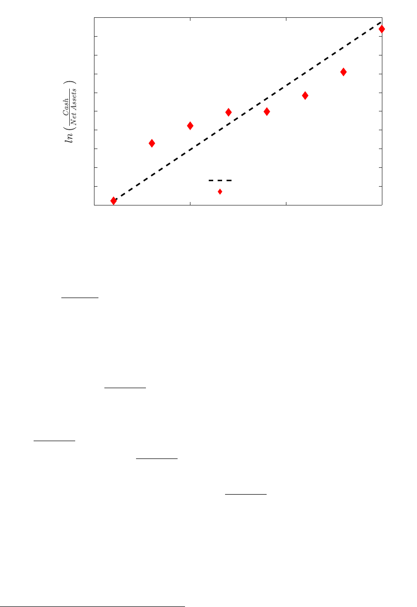
Figure 2: Foreign Liquid Asset Holdings and Eﬀective Repatriation Tax

Rates (Employment Weighted)

Notes: We follow the estimation in Foley, Hartzell, Titman, and Twite (2007), regressing foreign



Cash

Net Assets



on the employment-weighted-eﬀective repatriation tax rate and controls using our

simulated model data at the ﬁrm-level. The predicted values are generated by holding the control

variables at their conditional means. All values are centered at zero by subtracting the mean predicted

value. The slope of the dashed line follows the corresponding coeﬃcient estimate in Foley, Hartzell,

Titman, and Twite (2007) (Table 5, Column 3).

FHTT we calculate, for each ﬁrm, the employment-weighted-eﬀective repatriation tax rate.

We then regress ln



Cash

Net Assets



on the this weighted repatriation tax rate and the ﬁrm-level

controls used in FHTT.

Using the regression estimates from our simulated data, we generate predicted values

of ln



Cash

Net Assets



, holding the control variables at their conditional means. Figure 2 plots

the predicted values of ln



Cash

Net Assets



against the employment weighted repatriation tax rate

at evenly spaced intervals. In the ﬁgure, the predicted values are centered around zero by

subtracting the mean predicted value of ln



Cash

Net Assets



from each estimate. For comparison,

the dashed line follows the slope coeﬃcient estimate in FHTT.

Given we did not target this empirical relationship, this exercise (in addition to exercises

in forthcoming sections) provides conﬁdence in the external validity of our framework. More-

over, it also highlights an important channel through which repatriation taxes in the model

provide ﬁrms with a motive to hold ﬁnancial assets abroad. In the model, the stochastic

There are three control variables in FHTT for which our model does not have a counterpart: dividend

dummy (due to concave utility, ﬁrms always pay dividends in our model), R&D expenditures, and investment.

Details on this regression are in the Online Appendix.

element in repatriation tax rates, 

, induces ﬁrms to accumulate foreign ﬁnancial assets

to await tax saving from a lower realization of 

(therefore a lower τ

). Given positive

borrowing costs, when the underlying repatriation tax rate τ is high, the marginal utility of

shareholders from dividends is also relatively high. In this case, the marginal beneﬁt of tax

saving from a lower realization of 

is likewise high, leading ﬁrms to defer repatriations to

await such a realization. Additionally, recall that in the model foreign asset holdings reduce

domestic debt costs. Repatriation taxes thus induce ﬁrms to hold assets up to the point

where the marginal returns on after-tax repatriations equals the marginal cost of debt.

3.2.2 Asset Allocation and Production

Next, we look at the policy functions to understand the production and debt decisions

of the ﬁrm. We numerically solve for the policy functions for various levels of the debt-

elastic interest rate parameter ψ, holding ﬁrm-level productivity parameters, z

and z

and foreign asset holdings, A

, at their mean levels. We interpret ψ as the ease of access to

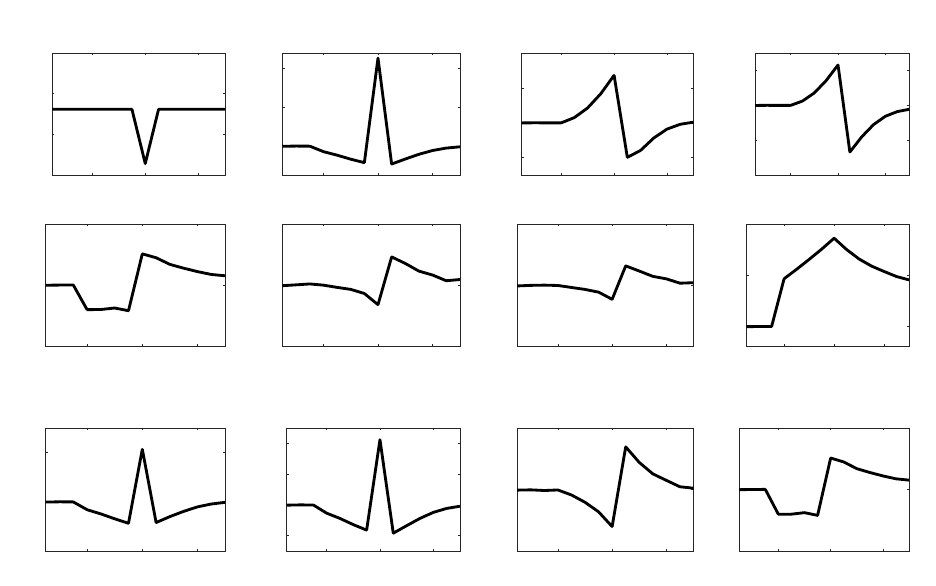
external credit markets. Figure 3 plots the policy functions for U.S. operations of internally

held assets, A

, against assets devoted to production, A

, ﬁnancial asset holdings, A

and U.S. proﬁts. Here A

< 0 indicates debt.

We let A

∗

denote the level of productive assets when the returns to production equal

the interest rate oﬀered by ﬁnancial asset holdings.

When A

< A

∗

the ﬁrm allocates

all of its internally held assets to production as these oﬀer a relatively higher return. Once

≥ A

∗

, production is at its maximum scale and, because of diminishing returns to scale

in production, all assets A

> A

∗

are held in interest bearing ﬁnancial assets.

Looking ﬁrst at the baseline parameterization of ψ, the total amount of assets devoted

to production is relatively unaﬀected by the amount of internally held assets A

. This

is because the ﬁrm may borrow to supplement its productive assets when the returns to

production exceed its borrowing costs (i.e. A

< 0 when A

< A

∗

). Proﬁts, although

growing in A

, are not substantially impacted by the level of internally held assets due to

the ﬁrm’s ability to access debt. Contrast this to the cases when it is more costly to access

external credit (or impossible when ψ = ∞).

When internally held assets A

< A

∗

the

amount of assets devoted to production – and thus proﬁts – are lower than the baseline case.

This is because it is more costly to supplement the shortfall in assets devoted to production

with debt.

These policy functions are instructive when understanding the model exercises of a re-

See Equation (20) in the Appendix for the solution to A

∗

U S

We note that the policy functions of foreign operations mirror the policy functions shown here when

ψ = ∞.

Figure 3: Policy Functions and Access to External Credit

duction in repatriation tax rates, which, we will see, lend to an inﬂux of foreign assets and

hence an increase in A

. As our policy functions illustrate, even large changes in A

our baseline case will have relatively small impacts on assets devoted to U.S. production

and, by extension, use of capital and labor.

4 Quantitative analysis

This section presents our model dynamics from a temporary repatriation tax rate reduction

– a tax holiday – where the ﬁrm receives news of the policy change in advance. We then

compare our model predictions with the empirical ﬁndings on the eﬀects of the tax holiday

around the American Jobs Creation Act of 2004. We show that the model is consistent

with this empirical literature and that it can account for a substantial share of the observed

repatriated assets before, during, and after the policy change. Following this, we examine the

importance of news, uncertainty, and access to external credit markets on ﬁrm-level behavior

stemming from a repatriation tax policy change.

4.1 Baseline Exercise

Our baseline experiment considers a tax holiday that reduces the repatriation tax rate faced

by multinational ﬁrms for one period from a steady state level of τ

to τ

. We further

assume that ﬁrms receive news of the tax holiday T periods in advance of its enactment.

This choice for the baseline tax policy is motivated by the American Jobs Creation Act of

2004 (AJCA), the only repatriation tax holiday in U.S. history. The AJCA contained several

tax incentives, including a one-time allowance for ﬁrms to bring back assets from abroad at

a reduced repatriation tax rate. For our baseline exercise, consistent with the AJCA, we

reduce repatriation tax rates for one-period from τ

= 0.131 to τ

= 0.0643.

In this exercise, the ﬁrm knows with certainty that a tax holiday will occur 4 periods

in advance of the actual tax holiday occurring, i.e. T = 4. Such policy lags are typical for

ﬁscal policy changes and are crucial to quantifying the full eﬀects of a tax holiday. In our

subsequent discussion, we refer to these policy lags – the periods between when the ﬁrm

begins anticipating a future tax holiday and when it is implemented – as the news periods.

Figure 4 presents the responses to news of, and implementation of, a tax holiday per

our baseline policy. The plots are the average responses of the multinational ﬁrms that we

model, and there is not economy-wide aggregation. Throughout, panels and results labeled

as “U.S.” refer to the average responses to U.S. variables. Panel A gives the ﬁrm-level

responses and panel B gives the responses for the U.S. government’s tax revenue collected

from these ﬁrms. The units are percentage deviations from the original stochastic steady

state with the exception of the repatriation tax rate graph, which shows the actual time-

path for the repatriation tax rate. The tax holiday is implemented at period 0 and the ﬁrm

receives news of it 4 quarters in advance (period -4).

It is most instructive to discuss our results by dividing the eﬀects of our baseline repa-

triation tax holiday into three separate sub-intervals: the news period (pre-realization, from

periods -4 to -1), the period of the tax holiday (at-realization, period 0), and the periods

thereafter (post-realization, period 1 onwards). On receiving news about an imminent future

tax holiday, during the news period the ﬁrm cuts back on repatriations from their foreign

subsidiary as they await more favorable repatriation tax rates. This leads to an accumu-

lation of ﬁnancial assets abroad. In the U.S., the ﬁrm compensates for this reduction in

transfers by issuing debt. However, since borrowing is not costless, the U.S. operations are

Under the AJCA, ﬁrms were allowed a maximum tax rate on overseas earnings of 5.25 percent on 85

percent of repatriated funds. The remaining 15 percent of funds faced their ‘normal’ repatriation tax rate,

0.131. The average repatriation tax rate on our model ﬁrms in the tax holiday is thus 0.85 × 0.0525 +

0.15 × 0.131 = 0.0643. Kleinbard and Driessen (2008) note that additional tax credits toward the eﬀective

tax rate on funds receiving tax breaks under the AJCA was 3.65 percent rather than 5.25 percent. Since we

do not explicitly model additional foreign tax credits, we use the 5.25 percent rate in our calculation.

-4 0 4

0.05

0.1

0.15

0.2

Repatriation tax rate

-4 0 4

200

400

Repatriations

-4 0 4

-100

100

200

Foreign financial assets

-4 0 4

-100

-50

U.S. debt

-4 0 4

-5

Dividends

-4 0 4

-1

U.S. labor and capital

-4 0 4

-1

U.S. output

-4 0 4

0.5

Firm value (V)

-4 0 4

-20

All sources

-4 0 4

-100

100

200

Repatriations

-4 0 4

-1

Corporate income

-4 0 4

-5

Dividends

Panel A: Firm-level responses

Panel B: US tax revenue by source

Figure 4: Responses to an Announced Temporary Reduction in Repatriation Taxes

Notes: News of tax reduction is received 4 quarters in advance. Except for the repatriation tax rate, units are in percent

deviation from initial steady state.

unable to fully make up for the entire fall in assets and thus have to cut back on dividend

payments and assets devoted to production. The fall in U.S. capital and labor is quite small

at approximately 3/10 of 1 percent.

In the period of implementation, the ﬁrm takes advantage of the one-time tax holiday

and repatriates a large amount of foreign assets to the U.S. The amount of repatriated assets

contains not only the ﬁnancial assets the ﬁrm accumulated abroad during the news period,

but to take maximum beneﬁt of the tax holiday the ﬁrm also brings forward planned future

transfers to the period of implementation. The U.S. operations then use this large inﬂow of

funds from abroad to pay higher dividends, reduce debt, and increase production.

After the tax holiday period, the ﬁrm reduces transfers and reaccumulates assets abroad

toward returning to their steady state level. In the U.S., the ﬁrm uses the large inﬂux of

assets from the tax holiday period to temporarily sustain higher dividend payments, higher

production, and debt reduction.

Next, with respect to share value and dividend payments, the announcement of a tax

holiday signals a lower tax obligation in the future, which causes an instant increase in the

ﬁrm’s value at the time of the news. The value of the ﬁrm continues to rise within the

news period up to the realization period, after which it slowly returns to steady state as

the tax-savings from the tax holiday are eventually paid out as dividends. Further, during

the news period, even though dividends are cut back they are still positive. When the ﬁrm

foresees a future tax reduction, they accumulate foreign ﬁnancial assets while simultaneously

issuing domestic debt to smooth out dividend payments. This behavior is consistent with

the observation that several companies (Apple Inc., Ford Motor Co., Caterpillar Inc., for

instance) have relied on bond issuance to ﬁnance dividend payments while simultaneously

amassing large sums of untaxed assets abroad.

On the U.S. government side, in Panel B, the collection of tax revenues on repatriated

assets, corporate income, and dividends mirror the transition path of their respective tax

sources.

The responses of tax revenues from corporate income and dividends are small

relative to that of transfers. Since the ﬁrm uses debt to smooth out U.S. production and

dividend payments, the magnitude of the impact from transfers is the primary force governing

the changes in tax revenues from all sources.

4.2 The American Jobs Creation Act of 2004

Our baseline calibration was informed by the actual tax rate reduction from the AJCA,

leading to a natural benchmark from which to judge the validity of our framework. Here we

compare our baseline results directly with the main ﬁndings from the empirical literature

that evaluates the impact of the AJCA.

Our model is able to explain key empirical ﬁndings

surrounding the AJCA. We also present suggestive evidence that ﬁrms both anticipated

and reacted to the tax holiday provision in the AJCA well before it was signed into law.

Furthermore, the eﬀects of policy lasted for several quarters after the end of the tax holiday.

This evidence lends support to the importance of accounting for the full dynamics in any

analysis of repatriation tax policy reform.

It is estimated that under the AJCA tax holiday approximately $312 billion of qualiﬁed

earnings were repatriated to the U.S. (Redmiles, 2008). Figure 5 shows net repatriated

dividends from foreign subsidiaries to U.S. based parent companies as a share of foreign

corporate proﬁts in the years around the AJCA. The shaded area is the eﬀective period of the

tax holiday

and the horizontal line - at 15% – is the average from 1995-2003. Net repatriated

Our model does not incorporate proﬁt shifting – attributing U.S. value added to foreign aﬃliates – for

tax purposes (see Guvenen, Mataloni Jr, Rassier, and Ruhl (2017)). If our model included opportunities for

proﬁt shifting, proﬁt shifting could increase if ﬁrms anticipate a repatriation tax rate reduction. While this

would not aﬀect real variables, it may amplify the responses to tax revenues.

A summary of this literature is in the Online Appendix. This literature, surprisingly, generally does

not consider the anticipatory eﬀects of repatriation tax policy changes.

Due to misalignment of ﬁscal to calendar years, some ﬁrms were allowed tax breaks on repatriated

income extending into 2006Q1.

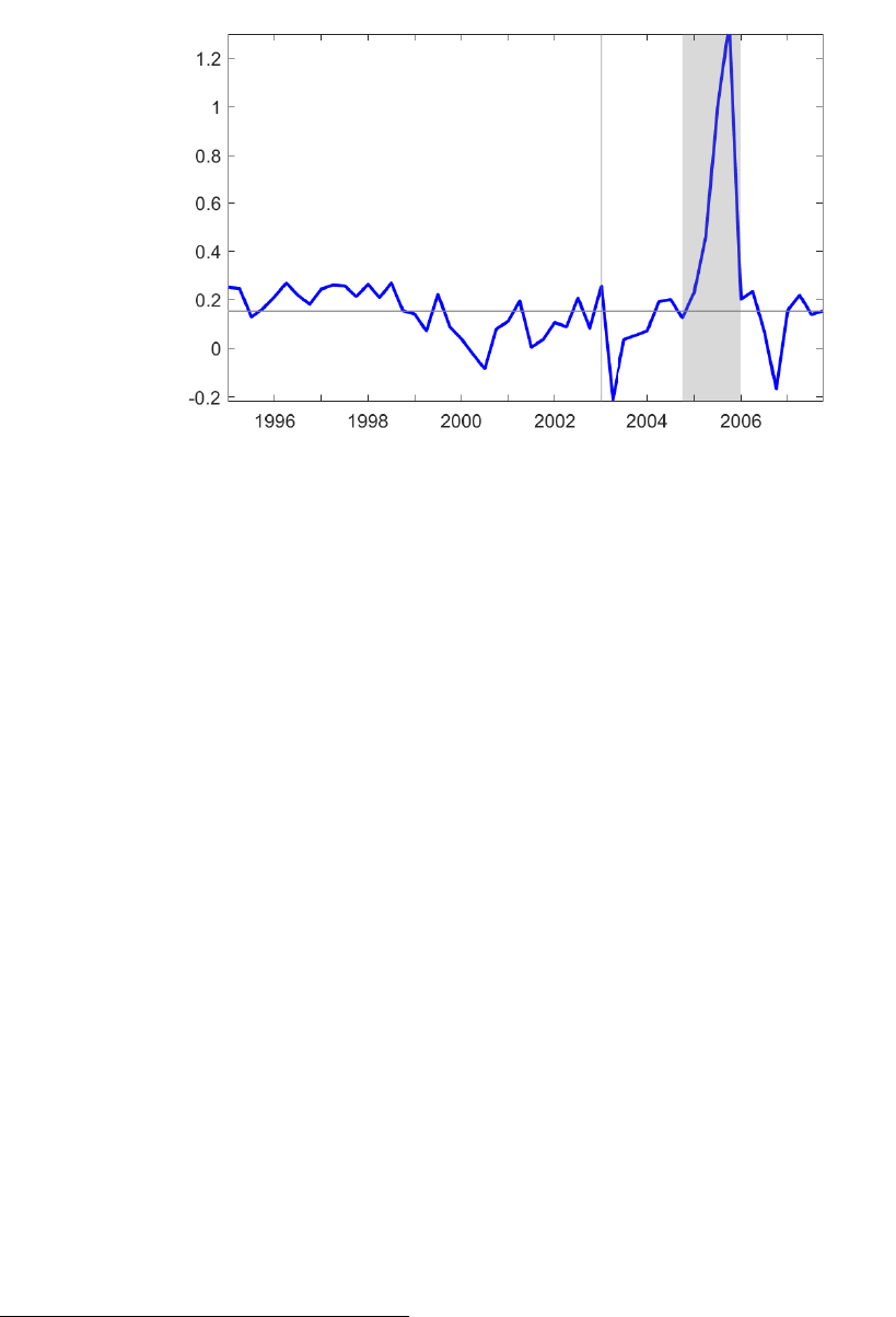
Figure 5: Transfers: Net Repatriations of U.S. Incorporated Companies

as a Share of Foreign Proﬁts

Notes: Constructed using Balance of Payments data from the U.S. Bureau of Economic Analysis

dividends as a share of corporate proﬁts had never exceeded 26% prior to the enactment of

the law, but reached 130% in the ﬁnal quarter of the tax holiday before sharply falling below

its average level just following the repatriation tax holiday. The fall in repatriations after the

tax holiday was anticipated by policy makers. The Joint Committee on Taxation predicted

ﬁrms would shift repatriated earnings they would otherwise have repatriated in future years

to the tax-holiday period to get more favorable rates (Kleinbard and Driessen, 2008). This

is the same mechanism that causes repatriations to fall after the tax holiday in our model.

Despite the inﬂux of liquidity during the tax holiday, the general consensus in the lit-

erature is that the AJCA’s objective of stimulating employment and investment were not

met. Dharmapala, Foley, and Forbes (2011) ﬁnd that repatriations had no signiﬁcant im-

pact on U.S. investment or employment, as did Clemons and Kinney (2008) with regards to

investment.

Faulkender and Petersen (2012) echo these ﬁndings and show that ﬁnancially

unconstrained ﬁrms, which repatriated 73% of all qualiﬁed funds, did not alter domestic

employment or investment.

Additionally, under the AJCA, funds receiving tax breaks were prohibited from being

used for shareholder payouts (dividends and share buybacks). However, in an evaluation of

the proposed tax holiday released a year prior to the AJCA, a Congressional Research Service

report noted that due to the fungibility of internal funds, ﬁrms could channel the repatriated

Further, of the top 15 repatriating corporations, 10 actually reported a decrease in U.S. jobs from

2004-2007 (Permanent Subcommittee on Investigations, 2011).

However, Faulkender and Petersen (2012) also document that ﬁnancially constrained ﬁrms did increase

investment, but still not employment, in response to the act. We return to this point in Section 4.5.

funds from a tax holiday to investment while switching domestic funds to shareholder payouts

(Brumbaugh, 2003). Studies on the AJCA have, in fact, found that the tax holiday was

associated with an increase in payments to shareholders (Blouin and Krull, 2009; Clemons

and Kinney, 2008). Dharmapala, Foley, and Forbes (2011) estimate that a $1 increase

in repatriation during the AJCA tax holiday corresponded with a $0.60–$0.92 increase in

shareholder payouts. In our model we can do a similar calculation. Relative to the steady

state, in the ﬁve-year window around the tax holiday (including the news period) in our

model, a $1 increase in after tax repatriations corresponds with a $0.74 increase in dividend

payouts. This is in the middle of the range found by Dharmapala, Foley, and Forbes (2011).

Studies on the impacts of the AJCA have primarily focused on its impact only at and

after its enactment. However, we argue that to correctly quantify the eﬀects of the AJCA,

one must also account for any anticipatory eﬀects that may have occurred, i.e. the impacts

during the news period. In the case of the AJCA, there were a series of earlier bills beginning

in February 2003 that did not pass through congress but contained the tax holiday provisions

that were later incorporated in the AJCA.

In the time leading up to the AJCA, there is evidence that these earlier bills did lead

to anticipation of the tax holiday. For example, in 2003 Lehman Brothers’ tax accounting

analyst Robert Wilkens indicated that legislation allowing companies to repatriate foreign

earnings was “gaining momentum” and was likely to be passed into law in early 2004 (Cor-

porate Financing Week, 2003). Other examples of anticipation of the tax holiday include

Simpson and Wells (2003) who discuss ﬁrms’ lobbying eﬀorts for a tax holiday in 2003 citing

provisions that would eventually be enacted in the AJCA and Sullivan (2004) who question

if foreign income shifting in the years leading up through 2002 are related to tax holiday

proposals in congress. Oler, Shevlin, and Wilson (2007) ﬁnd that in 2003, well before the

introduction and passage of the AJCA but when a future tax holiday seemed likely, stock

prices had started reﬂecting potential tax savings from a tax holiday. This is a result that is

mimicked by our model; stock prices rise in the news period in anticipation of a future tax

holiday (see Figure 4).

In our model, expectations of a reduction of repatriation tax costs lead ﬁrm to reduce

repatriations until the policy’s resolution. We ﬁnd that the behavior of ﬁrms, in the period

before the AJCA, was consistent with that anticipatory eﬀect. Returning to Figure 5, the

Lobbying eﬀorts had long called for tax breaks on repatriated income, but the call for a tax holiday

gained legitimacy in February 2003 with the introduction of the Homeland Investment Act of 2003 to the

House of Representatives, the Invest in America Act of 2003 presented to the House in March, and the Invest

in the USA Act of 2003 introduced in the Senate in the same month. These bills included similar provisions

for the tax holiday included in the AJCA of 2004. Under the AJCA of 2004, 85 percent of repatriated

earnings would qualify for tax exemptions, the same as in the Invest in the USA Act of 2003. A later bill

introduced in November 2003, The American Jobs Creation Act of 2003, also contained similar language.

Table 2: Cumulative Percent Deviation from Average Net

Repatriations as a Share of Foreign Proﬁts (Quarterly Rate)

Sub-Period

News Period AJCA Post-AJCA

(2003Q2-2004Q3) (2004Q4-2006Q1) (2006Q2-20017Q1)

Data -63.65 258.08 -53.43

Model -49.72 106.02 -61.89

notes: Figures are percent deviation of net repatriations as a share of foreign proﬁts relative

to their average. In the data, this is the average from 1995Q1-2003Q1. In the model the

average is the steady state level of the corresponding measure. Figures are expressed as

quarterly rates.

vertical line in 2003Q1 marks the time the ﬁrst bill leading up to the AJCA was introduced

(the Homeland Investment Act of 2003 ). The following quarter, net repatriated dividends

fell to their lowest point in the 13 year sample.

Table 2 compares our model ﬁndings with repatriation behavior in the data. We calculate

– in both the empirical and in the simulated data – the percent deviation of net repatriations

as a share of foreign proﬁts from its average level. We then cumulate it into 3 sub-periods:

6 quarters of the news period beginning with the introduction of the Homeland Investment

Act of 2003, 6 quarters of the eﬀective period of the AJCA, and 4 quarters after the policy.

All of the numbers are expressed as quarterly rates. For consistency in the comparison, we

rerun our baseline model but alter its timing to be consistent with the AJCA – a 6 quarter

news period and a 6 quarter tax holiday.

Quantitatively, the model matches the data very closely in the news period and in the time

following the tax holiday. During the tax holiday, in both the data and model, repatriations

are signiﬁcantly higher with the model capturing over 40 percent of this observed increase

during the AJCA. Overall, even though not constructed to explain the AJCA, our model is

able to account for various features of the data and the empirical results surrounding the

AJCA.

4.3 Discussion On General Equilibrium

While our focus is to understand the mechanisms driving within and cross-country asset

allocation of the ﬁrm in response to a change in repatriation taxes, before proceeding it

is important to note the limitations of our study when drawing aggregate implications.

Speciﬁcally, by lacking general equilibrium, our model economy does not capture indirect

eﬀects that may occur via price adjustments and/or changes in resource allocation.

In our model, as ﬁrms adjust their demand for inputs in response to the policy change,

input prices would adjust from changes in economy-wide demand. Likely, these price adjust-

ments in factor inputs would also serve to dampen the responses to labor/capital and output

in comparison to the already relatively small responses in our baseline model. Moreover, in

general equilibrium the asset ﬂows into the U.S. in response to a tax holiday would make

consumers wealthier – from an inﬂux of dividends and/or higher factor payments – and result

in an increase in demand for goods and services. Again, we would argue changes in factor

payments due to repatriations would be relatively small, causing the income and demand

change from this channel to be small. Dividend payments in our model, on the other hand,

fall in anticipation of, and increase at the time of, the tax change. The total eﬀects from this

channel would rely on how large the tax saving on dividends is and how large of a portion

dividend payments from multinational ﬁrms make up of total household income.

In the end, the aggregate responses would also depend on the extent to which wealth

eﬀects are assumed in household preferences. What is clear, however, is that the aggregate

and welfare eﬀects of repatriation taxes would necessitate a general equilibrium to be prop-

erly quantitatively evaluated. When we consider a permanent reduction in repatriation tax

rates, the general equilibrium eﬀects would be more important to incorporate as there may

exist long-run eﬃciency gains following a permanent reduction in distortionary taxes.

28,29

Our framework, nevertheless, highlights important mechanisms at the ﬁrm level that are

consistent with the empirical literature that such a framework should capture.

4.4 News Eﬀects

Policy analysis generally focuses on the eﬀects of a repatriation tax policy change only at

and after its enactment. For example, assessments of the AJCA such as the Joint Committee

on Taxation (2004) estimated the tax holiday provision in the AJCA would result in $2.8

billion in revenue gains during the holiday and over $6 billion in losses over the next 9 years.

The news period was not included in the assessment of the AJCA. In this section, we show

that the responses in the news period are large and, to ensure an accurate assessment of

any policy change, the entire dynamics surrounding the policy change should be taken into

account.

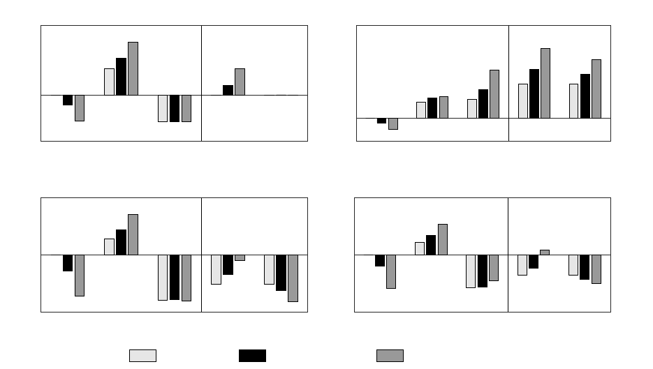
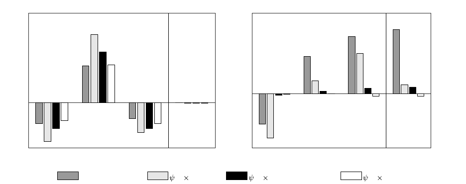
Figure 6 reports the cumulative responses of a tax holiday for several variables of interest.

Each plot also subdivides the cumulative responses into three sub-periods: pre-realization,

at-realization, post-realization. Additionally, we also report just the post-news cumulative

See, for example, Spencer (2017) for a general equilibrium model with permanent repatriation tax

changes.

Section OA5 of the Online Appendix considers a permanent reduction in repatriation taxes (and a

further discussion of general equilibrium eﬀects from this permanent change) as well as the permanent tax

reform from the Tax Cut and Jobs Act of 2017.

Repatriations

Pre At Post Post-news Total

-4

-2

Realization period Cumulative

U.S. labor and capital

Pre At Post Post-news Total

-0.005

0.005

0.01

0.015

0.02

Realization period Cumulative

U.S. repatriation tax revenue

Pre At Post Post-news Total

-3

-2

-1

Realization period Cumulative

U.S. tax revenue: all sources

Pre At Post Post-news Total

-0.4

-0.2

0.2

0.4

Realization period Cumulative

no news news period=1 news period=4 (baseline)

Figure 6: Cumulative Responses to a Tax Holiday

Notes: The cumulative eﬀects are shown news periods for when there is no news period and when the news period is 1 and 4

quarters long. The ﬁgures subdivide the cumulative responses in the three realization periods: Pre-realization, At-realization,

and Post-realization. This also shows the Post-news cumulative (sum of At- and Post-realization periods) and the total response

(sum of all subperiods). Units are quarterly gain/losses to that variable relative to the steady state at the time of the news.

response (the sum of the at-realization and post-realization responses) to highlight the im-

plications of a policy analysis that focuses only on the responses at and after a policy change.

For the ﬁgure, the units are quarterly gains/losses to that variable relative to the steady state

at the time of the news. For example, a cumulative value of -1 to tax revenues indicates

that total tax revenue losses are equal to 1 quarter’s worth of steady state tax revenues.

We further show the results for three simulations diﬀering in the length of the news period:

when there is no news period and when the news period is 1 and 4 quarters long.

Consider ﬁrst the cumulative impacts in the baseline case, i.e. news period is equal to 4.

On net, repatriations fall in the news period, rise during the tax holiday, and fall thereafter. If

an assessment of the tax holiday on repatriations only considers the total eﬀects at and after

its implementation, it shows a net gain of over 2 quarter’s worth of steady state repatriations.

When all periods are taken into account, including the news period, cumulative repatriations

are negligible: the policy change merely shifts the timing of transfers, which would have been

repatriated anyway, to the time of the tax holiday.

In the baseline case, there are cumulative gains to U.S. capital and labor. The total gains

to these variables are 1.3 percent of their quarterly steady state levels. If the news period

is not taken into account, these gains are overstated. On the government side, there are

net losses to U.S. tax revenues. However, looking at this set of ﬁrms, the tax holiday would

appear to be approximately revenue neutral if the news period were not taken into account.

Furthermore, we ﬁnd that the longer the news period the larger the losses to U.S. tax

revenue. A longer news period allows the ﬁrm to take maximum advantage of the tax holiday

by holding back a large amount of assets during the news period and then repatriating a

large amount during the tax holiday. This larger repatriation in turn leads to an overall

larger cumulative gain in the U.S. capital and labor, but at the same time also leads to

a larger revenue loss by the government. Thus, there is a tradeoﬀ between the length of

advanced notice and policy outcomes: a longer news period leads to higher cumulative gains

to employment but at the expense of larger tax revenue losses – although it should be noted

that the gains for labor and capital are quantitatively small while the losses in U.S. tax

revenue are relatively large. Put diﬀerently, if news periods are not taken into account

when analyzing the behavior of ﬁrms taking advantage of the tax holiday, policymakers may

overestimate the stimulative eﬀects of the policy and underestimate the costs in terms of tax

revenue losses by multinational ﬁrms.

4.5 Access to External Credit Markets

In this section we show that the magnitude of the response in a ﬁrm’s production activities,

given by ﬁrm-level capital and labor, is highly dependent on the level of access they have to

external credit.

Figure 7 shows the cumulative impacts of a one-period tax holiday under various values of

the parameter governing the ease with which ﬁrms can access to credit markets, ψ. Each ﬁg-

ure subdivides the responses into the pre-realization, at-realization, and the post-realization

periods. The cumulative response is the sum of the three sub-periods. Again, the units are

in quarterly gains/losses of that variable relative to the steady state. As in the baseline, the

temporary tax holiday reduces τ from 0.131 to 0.0642.

When the ﬁrm cannot access credit markets or the cost of borrowing is high, it relies

heavily on internal funds and thus the marginal value of an additional dollar in tax saving

from the upcoming tax holiday is high. Consequently, during the news period a credit

constrained ﬁrm aggressively cuts back transfers in order to take the maximum beneﬁts of

the tax holiday. The curtailing of transfers, in combination with the lack of access to cheap

credit, causes U.S. labor and capital to fall much more during the news period than in the

baseline case. On the other hand, a ﬁrm that has access to less costly borrowing also reduces

transfers in order to take advantage of the tax holiday. However, because they can borrow to

oﬀset this fall in transfers, there is little net eﬀect on U.S. labor and capital for these ﬁrms

during the news period. In comparison, there are large ﬂuctuations in labor and capital for

a credit-constrained ﬁrm at and after the tax holiday. These results are easy to understand

within the intuition provided by the policy functions shown in Section 3.2.2. In the presence

of low costs to external credit, ﬁrms are able to use debt to keep production close to its

optimal scale when internally held domestic assets (A

) fall due to the withholding of

transfers in the news period. Likewise, the scale of production is largely unchanged once the

policy change is implemented and foreign assets ﬂow into the U.S. (A

increases).

The labor and capital responses from our baseline model follow the empirical literature of

the AJCA. The majority of the ﬁrms receiving tax beneﬁts from the act were not ﬁnancially

constrained and therefore did not alter the scale of their U.S. operations (Dharmapala, Foley,

and Forbes, 2011; Faulkender and Petersen, 2012). Our baseline results reinforce these

ﬁndings. However, Faulkender and Petersen ﬁnd that a subset of ﬁrms that were ﬁnancially

constrained at the time of the AJCA did increase investment (but not employment) because

of the act. When analyzing the periods at and after the tax holiday, our model likewise

predicts that ﬁnancially constrained ﬁrms increase capital use after the holiday to a larger

degree than ﬁnancially unconstrained ﬁrms.

In general, our analysis shows why the ability of a ﬁrm to borrow can be very important

when understanding the eﬀects of future policy changes. For instance, Stokey (2016) shows

that tax uncertainty can generate an investment boon after the resolution of the uncertainty.

In her model, ﬁrms cannot borrow but can accumulate liquid assets. In the main exercise, a

Repatriations

Pre At Post Cumulative

-4

-2

U.S. capital and labor

Pre At Post Cumulative

-0.1

-0.05

0.05

0.1

0.15

No borrowing

=9 10

-2

=9 10

-4

(baseline) =9 10

-6

Figure 7: Cumulative Responses for Variations in Debt-Elastic Interest Rate Parameter, ψ

Notes: In the left panel a tax holiday is announced 4 periods in advance and in the right panel it is immediately and unexpectedly

implemented. The ﬁgures subdivide the cumulative responses in the three realization periods: Pre-realization, At-realization,

and Post-realization. The cumulative response is the sum of all subperiods. Units are quarterly gain/losses to that variable

relative to the initial steady state.

tax reform on revenue is announced that will be implemented at a known future date, but

the size of the tax rate change is uncertain. At the announcement of this future change, ﬁrms

reduce investment in new projects and accumulate liquid assets as a “wait and see” policy

until the uncertainty is resolved. When the tax reform is implemented, ﬁrms develop the

tabled projects and an upsurge in investment follows. Even though the exact characterization

of the tax reform and economy in Stokey (2016) diﬀers from our model, we can generate

similar investment dynamics. In our model, however, a reduction in domestic capital usage in

the news period and an upswing at the implementation of the tax holiday crucially depends

on restricting a ﬁrm’s access to credit markets. When ﬁrms can freely access external credit,

the domestic operations are already operating close to their optimal scale and a repatriation

tax rate reduction, or news surrounding such tax changes, has a negligible impact on domestic

production.

4.6 Policy Uncertainty

In the baseline simulations, ﬁrm know with certainty that a repatriation tax holiday is going

to occur at a known future date. However, in reality the legislative process is ripe with

uncertainty – ﬁrms are regularly uncertain about both if and when a policy being discussed

will be passed. In this section, we investigate the impacts of a tax holiday when there is

uncertainty in these dimensions.

4.6.1 When a Tax Holiday will Happen

Following the AJCA, ﬁrms steadily increased foreign asset holdings that were untaxed by

the U.S. government (Brennan, 2010). The AJCA was penned as a one-time event, but its

use as a stimulus measure may have altered expectations of the ability of policymakers to

enact a future repatriation tax holiday (Clausing, 2005; De Simone, Piotroski, and Tomy,

2017). Some have hypothesized that the accumulation of foreign assets after the AJCA was

due to expectations of another tax reduction at some point in the future (Levin and Coburn,

2011; Brennan, 2010). In our model, we ﬁnd if the ﬁrm believes a tax holiday will occur but

is uncertain about when it will occur, they steadily accumulate assets abroad.

Suppose the model ﬁrm receives news that a repatriation tax rate reduction will happen

at an unknown date between the time of the news and a given time T in the future. Further,

in each time period the ﬁrm assigns an equal probability that the tax change will occur in

each remaining period through period T .

We set T = 20 and in Figure 8 plot the foreign

ﬁnancial asset holdings during the news period. The size of the tax rate reduction is the

See the Online Appendix for a transition graph outlying this experiment.

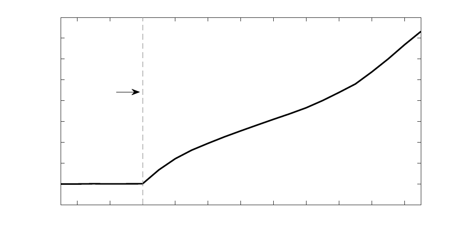
-24 -22 -20 -18 -16 -14 -12 -10 -8 -6 -4

-20

100

120

140

160

% deviation from steady state

News

Figure 8: Response to Foreign Financial Assets to a Temporary Reduction in the Repatriation

Tax Rate When the Date of Implementation is Uncertain

Notes: The ﬁrm receives news that a tax holiday will occur in the next 20 quarters but are unsure of the arrival date. The tax

holiday is arbitrarily chosen to occur after 18 periods. The expectations in the timing of the tax holiday are uniform across all

remaining periods if the tax holiday has not yet occurred. The ﬁgure shows up to two periods before the tax holiday occurs to

highlight the accumulation of foreign ﬁnancial assets prior to the holiday.

same as in the baseline. In these simulations, we arbitrarily let the implementation of the

tax reform to occur 18 quarters after receiving the news (t = −2). We do not show the

periods at and after the tax reductions to highlight the run up of foreign assets in the news

periods.

At the time of the news, the ﬁrm begins gradually accumulating foreign ﬁnancial assets.

After 17 quarters, these asset holdings are nearly 150 percent higher than their steady state

level. Since the timing of the policy change is unknown, the ﬁrm accrues these assets to take

advantage of tax gains that will occur once the tax holiday is implemented in the future.

Our model suggests that there may be merit to the conjecture that ﬁrms began accumu-

lating assets abroad in anticipation of a future repatriation tax reduction after the AJCA.

This relates to De Simone, Piotroski, and Tomy (2017) who ﬁnd that many multinational

ﬁrms accumulated foreign liquid assets in anticipation of a proposed, but failed, 2008 tax

holiday. Arguing that the AJCA changed expectations of the likelihood of similar policy

change, proposed legislation in 2008 for another tax holiday that never materialized may

have been a catalyst for many multinationals to accumulate assets abroad. In this regard,

our model suggests that at least part of the asset buildup abroad following the AJCA may not

be from a high steady state repatriation tax rate, but may be the direct result of discussions

and anticipation of a future repatriation tax rate reduction.

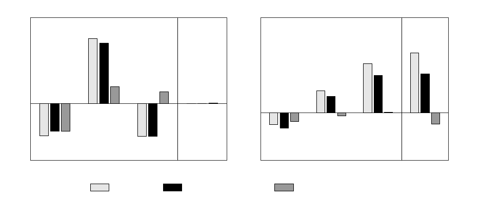
Repatriations

Pre At Post Cumulative

-4

-2

U.S. labor and capital

Pre At Post Cumulative

-0.01

-0.005

0.005

0.01

0.015

0.02

Baseline If (news materializes) If (news does not materialize)

Figure 9: Cumulative Responses When There is a 50 Percent Probability of the Tax Holiday

Occurring in 4 Quarters in Advance of the News

Notes: The ﬁgure shows the cases when the tax holiday does materialize and when it does not materialize along with the

baseline when the tax holiday occurs with certainty. The ﬁgures subdivide the cumulative responses in the three realization

periods: Pre-realization, At-realization, and Post-realization. The cumulative response is the sum of all sub-periods. Units are

quarterly gain/losses to that variable relative to the initial steady state.

4.6.2 If a Tax Holiday May Happen

Next, let us consider the case where the ﬁrm is unsure if a tax holiday will occur. In this

example, the ﬁrm receives news that in 4 quarters a one-period repatriation tax reduction

might occur. After 4 quarters of receiving the news, two outcomes are possible: the news

materializes whereby the repatriation tax rate is reduced as in the baseline, or the news

does not materialize and the ﬁrm realizes a tax holiday will not occur. In the following

simulations, the ﬁrm assigns a 50/50 likelihood of either outcome occurring.

Figure 9 shows the cumulative responses in each sub-period – pre, at, and post realization

– and the sum of all periods. The cases of uncertainty of if the tax holiday will occur (and

if it does or not happen) are compared against the baseline where the tax holiday occurs

with certainty. If the news materializes, the ﬁrm repatriates additional funds by transferring

assets that would otherwise be repatriated in future periods to the time of the tax holiday.

In contrast, when the tax holiday does not occur the ﬁrm has no such motive. Instead,

they simply repatriate the funds they accumulated in the news period. Overall, if the ﬁrm

anticipates the possibility of a future tax holiday and it does not occur, the cumulative eﬀects

are negligible. However, the mere prospect of a repatriation tax holiday disrupts the timing

of repatriation decisions.

4.7 Quantifying News and Uncertainty Eﬀects: the Shadow Tax

The prospect of a future repatriation tax reduction allows ﬁrms to take advantage of the

tax holiday by holding assets abroad and reducing repatriations. Thus, news of a possible

repatriation tax reduction actually generates an implicit tax – or shadow tax – on repatriating

funds during the news period. In our model, we can measure this shadow tax as the subsidy

rate the government will have to pay the ﬁrm in the period of receiving the news to encourage

them to not hold back repatriations in this period, and keep them at the original steady state

level. That is, how much would the U.S. government have to subsidize transfers by to induce

the ﬁrm to keep their level of transfers unchanged in response to news of a tax holiday?

We calculate the shadow tax under various scenarios and show that this implicit tax

depends on both the length of the news period and the degree of certainty of if and/or

when a tax holiday will occur. In panel A of Table 3, the ﬁrm receives news of a one-time

repatriation tax holiday that may occur in exactly T quarters from the news. We consider

two cases: one in which there is a 50 percent probability the tax holiday will happen and the

other where the tax holiday will happen with certainty. If the tax holiday is implemented,

the repatriation tax rate reduction is the same as the baseline.

Our shadow tax measure quantiﬁes the degree to which news of a repatriation tax reduc-

tion induces ﬁrms to accumulate foreign assets. It is growing in the likelihood of the passage

of a tax holiday and shrinking in the time until the realization of the news. The motive to

increase foreign asset holdings by reducing transfers at the time of the news is higher when

the passage of the tax holiday is likely and when ﬁrms have less time to amass these assets

in preparation for the possible tax holiday.

Table 3: Shadow Tax

Panel A: Certainty when news materializes Panel B: Uncertainty when news materializes

News material-

izes in T quar-

ters

P (if tax holiday)

News material-

izes within T

quarters

P (if tax holiday)

0.5 1 0.5 1

T = 1 2.67 5.49 T = 1 2.67 5.49

T = 2 2.08 4.58 T = 2 2.73 4.68

T = 3 1.47 3.61 T = 3 2.67 4.51

T = 4 0.90 1.95 T = 4 2.24 3.72

Notes: Units are in percent. The shadow tax is the subsidized rate on a ﬁrm’s repatriations at the time they receive news of a

potential tax holiday that would keep transfers constant at their original steady state level in that period. In panel A the ﬁrm knows

with certainty that a tax holiday will occur with a probability of 0.5 and 1 in exactly T periods. In panel B, the ﬁrm knows that a

tax holiday will occur with a probability of 0.5 and 1 at some period within T periods.

Turning next to panel B of Table 3, the ﬁrm receives news of a one-time repatriation tax

holiday that may occur with an unknown arrival date between the time of the news and T

quarters from the news. At each time period, the ﬁrm assigns an equal probability that the

tax change will occur in each of the remaining periods. We consider two cases, one where

there is a 50/50 chance the tax holiday will occur and one where the tax holiday will occur

with certainty. When T = 1, the exercises in panels A and B are identical. Comparing

pairwise with panel A for T > 1, the shadow tax with uncertainty in when the news will

materialize is always larger. When there is certainty that the arrival date is more than one

quarter out, the ﬁrm can wait to accumulate foreign assets right before the tax holiday. On

the other hand, when the ﬁrm is uncertain when the news will materialize, the motive of the

ﬁrm to accumulate foreign assets at the time of the news is larger as they prepare for the

chance the tax holiday may occur at any time.

In summary, news of a potential tax change is akin to levying an additional tax on

repatriated earnings in the periods leading up to the possible policy change. Our model shows

that, conditional on the probability that a repatriation tax holiday will occur, uncertainty

in the timing of when the tax holiday may be implemented increases the shadow tax on

repatriated foreign earnings. More generally, if discussions or proposals in congress alter the

probability distribution of the tax environment, then the news itself may act as an implicit

tax, with uncertainty about when the actual policy change will occur increasing this implicit

tax.

5 Conclusion

This paper presents a model of a multinational ﬁrm to understand how changes in repatria-

tion tax policy impact ﬁrm-level behavior. We discipline our framework with both aggregate

and ﬁrm-level data and use the American Jobs Creation Act of 2004 to test its external

validity. Our analysis serves to highlight the importance of understanding the dynamics

around, and timeliness in, resolving repatriation tax policy.

We ﬁnd that a policy evaluation that does not account for ﬁrm-level behavior before the

policy change overestimates the beneﬁts of reducing repatriation tax rates – by overstating

both the gains to domestic production activity and the amount of assets transferred from

abroad – and underestimates its costs by understating tax revenue losses. Additionally, the

length of the news period and policy uncertainty of when and if a tax change will occur

all have signiﬁcant eﬀects on the impact of a policy change. Furthermore, we show that

a ﬁrm’s access to external ﬁnancing plays an important role in determining the impact of

repatriation tax changes on domestic activity. Firms that have low costs of accessing external

credit markets can operate at their eﬃcient scale independent of access to foreign funds, and

are thus not materially aﬀected by changes in the repatriation tax rate. In other words, the

less credit constrained the ﬁrm is, the more muted the responses of real variables are to both

expected and realized changes in repatriation taxes.

In the time leading up to and after the AJCA, lawmakers actively discussed policies

to lower repatriation tax rates. A widely stated aim of these reforms was to encourage

U.S. based ﬁrms to repatriate foreign asset holdings. News of a potential reduction in

repatriation tax rates, which may arise from policy discussions, generates a wedge that

distorts the intertemporal cost of repatriating foreign assets. This wedge, or “shadow tax,”

on repatriating foreign earnings discourages ﬁrms to transfer income back to the US, thereby

leading to an accumulation of assets abroad. The shadow tax is further magniﬁed with

uncertainty regarding the timing of the policy’s resolution.

Even though lawmakers’ goals of lowering the repatriation tax rate was to encourage the

transfer of assets from abroad, expectations and uncertainty generated by their discussions

can have the opposite eﬀect by decreasing the incentives for ﬁrms to repatriate earnings until

the resolution of the policy discussion. Although unexplored in this paper, it may be that

revenue losses during this period are suﬃciently large such that lawmakers have the incentive

to implement a tax reduction. In other words, public discussions that indicate the intention

of changing repatriation tax policy could be self-fulﬁlling.

Appendix: Solution Method

In this section we outline the solution method. We proceed in three steps:

Step 1: Value Function

To solve the ﬁrm’s problem, we begin by using value function iteration to numerically con-

struct the value function given by (19). Our value function is deﬁned on a 6-dimensional

discrete grid that represents the state space, (A

, A

, τ, 

, z

). To interpolate values

of the value function along the A

×A

dimensions we use a combination of shape-preserving

Schumacher quadratic splines and linear splines on a 61×121 point discrete grid.

For the

shocks 

, z

, and z

we deﬁne a 7×9×9 grid and only consider values on the grid. We

set 

to be a discrete uniform random variable, while the discrete versions of the AR(1)

processes for z

and z

are calculated using Tauchen (1986)’s method. Finally, the grid

points for τ depend on the structure of the policy being evaluated. For example, for our

See Judd (1998).

baseline model where the news occurs after N = 4 periods, τ is deﬁned on N = 6 grid

points, corresponding to the 6 states of the economy – the pre- and post-policy steady-state

state, a state each for the 4 news periods, and a state for the period is which the policy is

implemented. In total, for our baseline model our value function is numerically represented

by approximately 25 million grid points.

The value function iteration requires a maximization step. After substitution, the four

dimensional maximization step, {A

, A

, T, d}, can be reduced to a maximization step in

just two dimensions, {A

, T }. We numerically maximize over these two variables using

two-dimensional Golden-section search.

Finally, to construct the value function we must also ﬁnd Π

and Π

. Whereas a closed

form solution exists for Π

, no closed form solution exists for Π

. The closed-form solution

to Π

is as follows:











1,F

α+η

+ τ

if A

< A

∗

2,F

+ [1 + (1 − τ

)r] (A

− A

∗

) if A

≥ A

∗

where

1,F

= (1 − τ

) e











α + η



α+η

2,F

= {(1 − τ

) (1 − α − η) (1 + r) + [1 + (1 − τ

)r] (α + η)}



1 + r











1−α−η

∗

= (α + η)



1 + r











1−α−η

Here A

∗

gives the level of assets where if all the ﬁrm’s assets were allocated to production

then the returns on them would equal the interest rate oﬀered by ﬁnancial asset holdings.

Due to diminishing returns, assets in excess of A

∗

allocated to production will earn a return

lower than that oﬀered on ﬁnancial assets, thus when A

≥ A

∗

the ﬁrm allocates (A

− A

∗

)

to ﬁnancial holdings and A

∗

to production.

For Π

, as no closed form solution exists, we construct numerical solutions for the grid

points in the A

, A

, and z

dimensions. This solution is constructed as follows:











if A

< A

∗

2,US

+ [1 + (1 − τ

)¯r] (A

− A

∗

) if A

≥ A

∗

where

2,US

= {(1 − τ

) (1 − α − η) (1 + r) + [1 + (1 − τ

)r] (α + η)}



1 + r











1−α−η

∗

= (α + η)



1 + r











1−α−η

. (20)

As before, A

∗

gives the level of assets where if all the ﬁrm’s assets were allocated

to production the returns on them would equal the interest rate oﬀered on ﬁnancial asset

holdings. Due to diminishing returns, assets in excess of A

∗

allocated to production will

earn a return lower than that oﬀered on ﬁnancial assets, thus when A

≥ A

∗

the ﬁrm

allocates (A

− A

∗

) to ﬁnancial holdings and A

∗

to production.

Next, to ﬁnd

we simplify and write Π

in terms of a maximization problem in L

and K

only.

= max



(1 − τ

+ (1 + r

)(A

− wL

− r

) + τ



where,

= r + ψ



exp



− wL

− r



− 1



We can solve this maximization problem by ﬁrst substituting in K

= (

)(

, which

we get from the ﬁrst-order conditions, and then use golden-section search to numerically ﬁnd

the optimal L

and thus

itself.

Step 2: Policy Functions

We use the value function found in the previous step to ﬁnd the policy functions:

= g

, A

, τ, 

, z

)

= g

, A

, τ, 

, z

Finding the policy functions, similar to the value function iteration, requires a maximization

step. As before, we reduce the four dimensional maximization step {A

, A

, T, d} to a

maximization step in just two dimensions, {A

, T } and use two-dimensional Golden-section

search.

We know this because in this case A

U S

< A

∗

U S

, which means the returns to assets allocated to production

are higher than r leading the ﬁrm to borrow (i.e. A

U S

< 0).

Our policy functions is deﬁned on a 6-dimensional discrete grid that represents the state

space, (A

, A

, τ, 

, z

). At 501×501, this grid is ﬁner than the value function in

the A

and A

dimensions. We do not interpolate between these points and impose the

condition that A

and A

must also lie on the grid. Thus, for our baseline model our

policy functions are numerically represented by approximately 850 million grid points that

map onto a roughly 250 thousand grid point values for (A

, A

Step 3: Simulations

Finally, we use the policy functions constructed in Step 2 to simulate the economy. To

construct the response of the economy to various policies we simulate our environment for

700 periods with the tax news arriving in period 600. We repeat this 700 period simulation

200,000 times keeping the tax news the same but allowing the idiosyncratic shocks 

, z

and z

to vary. We then average across these 200,000 simulations. We include 600 period

before the tax news to allow the economy to settle into its stochastic steady state.

References

Altshuler, R. and H. Grubert (2003): “Repatriation Taxes, Repatriation Strategies

and Multinational Financial Policy,” Journal of Public Economics, 87, 73–107.

Beaudry, P. and F. Portier (2007): “When Can Changes in Expectations Cause Busi-

ness Cycle Fluctuations in Neo-Classical Settings?” Journal of Economic Theory, 135,

458–477.

Bloom, N. (2009): “The Impact of Uncertainty Shocks,” Econometrica, 77, 623–685.

Blouin, J. and L. Krull (2009): “Bringing it Home: A Study of the Incentives Sur-

rounding the Repatriation of Foreign Earnings Under the American Jobs Creation Act of

2004,” Journal of Accounting Research, 47, 1027–1059.

Brennan, T. J. (2010): “What Happens After a Holiday? Long-term Eﬀects of the Repa-

triation Provision of the AJCA,” Northwestern Journal of Law and Social Policy, 5, 1.

Brumbaugh, D. (2003): “Tax Exemption for Repatriated Foreign Earnings: Proposals and

Analysis,” Congressional Research Service, Library of Congress.

Clausing, K. A. (2005): “Tax Holidays (and other escapes) in the American Jobs Creation

Act,” National Tax Journal, 331–346.

Clemons, R. and M. Kinney (2008): “An Analysis of the Tax Holiday for Repatriation

Under the Jobs Act,” Tax Notes, 120.

Corporate Financing Week (2003): “Repatriation Bill Gathers Momentum,” October

27.

De Simone, L., J. D. Piotroski, and R. E. Tomy (2017): “Repatriation Taxes and

Foreign Cash Holdings: The Impact of Anticipated Tax Reform,” The Review of Financial

Studies.

De Waegenaere, A. and R. C. Sansing (2008): “Taxation of International Investment

and Accounting Valuation,” Contemporary Accounting Research, 25, 1045–1066.

Dharmapala, D., C. F. Foley, and K. J. Forbes (2011): “Watch What I do, Not What

I Say: The Unintended Consequences of the Homeland Investment Act,” The Journal of

Finance, 66, 753–787.

Faulkender, M. and M. Petersen (2012): “Investment and Capital Constraints: Repa-

triations Under the American Jobs Creation Act,” Review of Financial Studies, 25, 3351–

3388.

Foley, C. F., J. C. Hartzell, S. Titman, and G. Twite (2007): “Why Do Firms

Hold So Much Cash? A Tax-Based Explanation,” Journal of Financial Economics, 86,

579–607.

Graham, J. R. (1996): “Proxies for the Corporate Marginal Tax Rate,” Journal of Finan-

cial Economics, 42, 187–221.

Gu, T. (2017): “US Multinationals and Cash Holdings,” Journal of Financial Economics,

125, 344–368.

Guvenen, F., R. J. Mataloni Jr, D. G. Rassier, and K. J. Ruhl (2017): “Oﬀ-

shore Proﬁt Shifting and Domestic Productivity Measurement,” NBER Working Paper

No. 23324.

Hartman, D. G. (1985): “Tax Policy and Foreign Direct Investment,” Journal of Public

Economics, 26, 107–121.

House, C. L. and M. D. Shapiro (2006): “Phased-in Tax Cuts and Economic Activity,”

The American Economic Review, 96, 1835–1849.

Joint Committee on Taxation (2004): “Estimated Budget Eﬀets of the Conference

Agreement for H.R. 4520, The ‘American Jobs Creation Act of 2004’,” JCX-69-04, Joint

Committee on Taxation, Washington D.C.

Judd, K. L. (1998): Numerical Methods in Economics, MIT press.

Kleinbard, E. D. and P. Driessen (2008): “A Revenue Estimate Case Study: The

Repatriation Holiday Revisited,” Tax Notes, 120.

Leeper, E. M., A. W. Richter, and T. B. Walker (2012): “Quantitative Eﬀects of

Fiscal Foresight,” American Economic Journal: Economic Policy, 4, 115–144.

Levin, C. and T. Coburn (2011): “Repatriating Oﬀshore Funds: 2004 Tax Windfall for

Select Multinationals,” United States Senate Permanent Subcommittee on Investigations,

11.

Matheson, T., V. Perry, and C. Veung (2013): “Territorial vs. Worldwide Corporate

Taxation: Implications for Developing Countries,” IMF Working Paper: Territorial vs.

Worldwide Corporate Taxation-Implications for Developing Countries, 13.

Mertens, K. and M. O. Ravn (2011): “Understanding the Aggregate Eﬀects of Antici-

pated and Unanticipated Tax Policy Shocks,” Review of Economic Dynamics, 14, 27–54.

Oler, M., T. Shevlin, and R. Wilson (2007): “Examining Investor Expectations Con-

cerning Tax Savings on the Repatriations of Foreign Earnings Under the American Jobs

Creation Act of 2004,” Journal of the American Taxation Association, 29, 25–55.

Permanent Subcommittee on Investigations (2011): Repatriating Oﬀshore Funds:

2004 Tax Windfall for Select Multinationals, U.S. Senate Committee on Homeland Security

and Governmental Aﬀairs, October 11.

Redmiles, M. (2008): “The One-Time Dividends Received Deduction,” IRS Statistics of

Income Bulletin, 27, 102–114.

Schmitt-Groh

e, S. and M. Uribe (2003): “Closing Small Open Economy Models,”

Journal of international Economics, 61, 163–185.

Simpson, G. R. and R. Wells (2003): “Firms Accused of Using Shelters Lobby

U.S. to Repatriate Funds,” The Wall Street Journal, accessed June 20, 2016:

http://www.wsj.com/articles/SB105329431199082400.

Spencer, A. (2017): “Policy eﬀects of international taxation on ﬁrm dynamics and capital

structure,” Working Paper.

Stokey, N. L. (2016): “Wait-and-See: Investment Options Under Policy Uncertainty,”

Review of Economic Dynamics, 21, 246–265.

Sullivan, M. (2004): “Data Show Dramatic Shift of Proﬁts to Tax Havens,” Tax Notes,

13, 1190–1200.

Tauchen, G. (1986): “Finite state markov-chain approximations to univariate and vector

autoregressions,” Economics letters, 20, 177–181.

van’t Riet, M. and A. Lejour (2014): “Potential Beneﬁts of Tax Inversion Remain

(Huge): with the model and full country rankings,” CPB Netherlands Bureau for Economic

Policy Analysis Backround Document.

Yang, S.-C. S. (2005): “Quantifying Tax Eﬀects Under Policy Foresight,” Journal of

Monetary Economics, 52, 1557–1568.

Online Appendix for “Repatriation Taxes”

(Not For Publication)

This not-for-publication appendix contains additional analysis of our framework.

Contents

OA1 Transition Probabilities for Experiments 2

OA1.1 Baseline . . . . . . . . . . . . . . . . . . . . . . . . . . . . . . . . . . . . . . . . . 2

OA1.2 Uncertainty: When a Tax Holiday May Occur . . . . . . . . . . . . . . . . . . . 2

OA1.3 Uncertainty: If a Tax Holiday May Occur . . . . . . . . . . . . . . . . . . . . . . 3

OA1.4 Uncertainty in If and When a Tax Holiday May Occur . . . . . . . . . . . . . . . 4

OA2 Model Comparison with Foley, Hartzell, Titman, and Twite (2007) 5

OA3 Additional Evidence of News: Permanently Reinvested Earnings and the

AJCA 6

OA4 AJCA Literature and Model Comparison 8

OA5 Sensitivity Analysis 10

OA5.1 Shareholder Preferences . . . . . . . . . . . . . . . . . . . . . . . . . . . . . . . . 10

OA5.2 Foreign Borrowing . . . . . . . . . . . . . . . . . . . . . . . . . . . . . . . . . . . 11

OA5.3 Permanent Repatriation Tax Cut . . . . . . . . . . . . . . . . . . . . . . . . . . 12

OA5.4 Discussion On General Equilibrium . . . . . . . . . . . . . . . . . . . . . . . . . 14

OA6 Tax Cut and Jobs Act of 2017 15

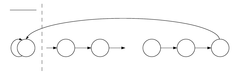
OA1 Transition Probabilities for Experiments

This appendix describes the ﬁrm’s expectations of future policy from the period of receiving news

through the resolution of the news.

OA1.1 Baseline

In the baseline simulations, the ﬁrm unexpectedly receives a tax news shock that notiﬁes them

that there will be a one-period repatriation tax rate reduction 4 quarters in the future. Figure A1

shows the transition graph for the general case when the time from the news to the tax holiday is

T quarters. After the tax holiday, the repatriation tax rate returns to its original steady-state rate

indeﬁnitely.

…

Steady State

Tax

News

Tax

Holiday

Prob = 1

Period 1 Period 2

Period T–2

Steady

State

Prob = 1 Prob = 1 Prob = 1 Prob = 1

Prob = 1

Period T–1

Figure A1: Transition Graph for Baseline Simulation: Tax Holiday Occurring T Periods From

the Arrival of the News

OA1.2 Uncertainty: When a Tax Holiday May Occur

Figure A2 shows the transition graph for the case when ﬁrms receive news of a one-period temporary

repatriation tax reduction that will occur at an unknown time between the arrival of the news and

T periods from the arrival of the news. This corresponds to the simulations in Section 4.5.1 in the

main text. If the tax holiday has not occurred in a given period, the ﬁrm places an equal likelihood

that the tax holiday will occur in any given future period. For example, if T = 8, then in the ﬁrst

period of the news ﬁrms will place a P

= 1/8 probability that it will occur in the next period,

and if it doesn’t occur in the next period then in period 2 they place a P

= 1/7 probability of it

occurring in the following period, and so on. Once the tax holiday occurs, the repatriation tax rate

returns to its original steady-state rate indeﬁnitely.

…

Steady State

Tax

News

Tax

Holiday

Prob =

1 – P

Prob =

1 – P

Prob =

1 – P

T-2

Prob = 1

T-2

Prob = P

Period 1 Period 2

Steady

State

Prob = 1

Period T–2 Period T–1

Figure A2: Transition Graph With Uncertainty of When a Tax Holiday May Occur Between

the Arrival of the News and T Periods Afterwards

OA1.3 Uncertainty: If a Tax Holiday May Occur

Figure A3 shows the transition graph for the case when ﬁrms receive news of a one-period temporary

repatriation tax reduction that may or may not occur T periods in the future. This corresponds

to the simulations in Section 4.5.2 in the main text. The ﬁrm unexpectedly receives a tax news

shock that notiﬁes them there may be a temporary repatriation tax rate reduction T quarters in

the future. At time T − 1, the ﬁrm knows that the tax news will be resolved with a probability

of the tax holiday occurring as P (Occur) and probability 1 − P (Occur) that it will not occur. If

the tax holiday does occur, the ﬁrm will receive a one-period repatriation tax reduction before the

repatriation tax rate returns to the original steady-state rate indeﬁnitely. If it does not occur, the

repatriation tax rate returns to its original steady-state rate indeﬁnitely.

…

Steady State

Tax

News

Tax

Holiday

Prob = 1

Period 1 Period 2

Steady

State

Prob =

P(Occur)

Prob = 1 Prob = 1 Prob = 1

Prob = 1

Prob = 1 – P(Occur)

Period T–2 Period T–1

Figure A3: Transition Graph With Uncertain Tax Holiday Occurring T Periods From Arrival

of the News

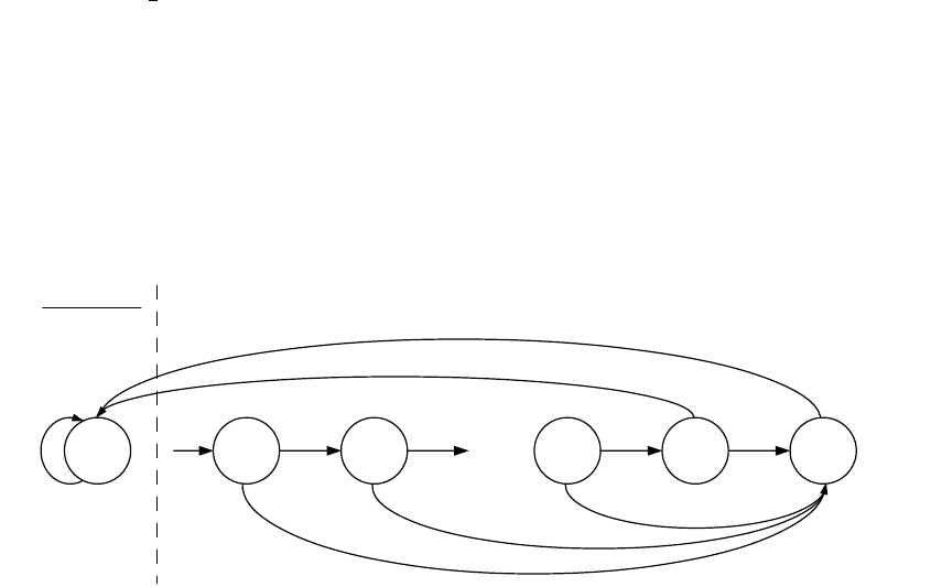
OA1.4 Uncertainty in If and When a Tax Holiday May Occur

Section 4.6 in the main text reports the shadow tax on repatriated earnings at the period the

ﬁrm receives news of a possible repatriation tax holiday. Figure A4 shows the general case of the

transition graph used in calculating these shadow taxes. The ﬁrm receives news of a temporary

repatriation tax reduction that may or may not occur between the arrival of the news and T periods

from the arrival of the news. If the tax holiday has not occurred in a given period, the ﬁrm places

an equal likelihood that the tax holiday may occur in any given future period. They additionally

place a probability that the holiday will occur at all (P (Occur) = P

T −1

). For example, if T = 4

and ﬁrms place a 50 percent probability a tax holiday will occur, then in the ﬁrst period of the

news ﬁrms place a

× 0.5 probability it will occur in the next period and in each remaining period.

At time T − 1, ﬁrms know that the tax news will be resolved with a probability of the tax holiday

occurring as P

T −1

and probability 1 − P

T −1

that it will not occur. If the tax holiday does occur,

the ﬁrm receives a one-period repatriation tax reduction before the repatriation tax rate returns to

its original steady-state rate indeﬁnitely. If it does not occur, the repatriation tax rate returns to

its original steady-state rate indeﬁnitely.

…

Steady State

Tax

News

Tax

Holiday

Prob =

1 – P

Prob =

1 – P

Prob =

1 – P

T-2

Prob = 1 – P

T-1

Prob = 1

T-1

Prob = P

T-2

Prob = P

Period 1 Period 2

Steady

State

Prob = 1

Period T–1Period T–2

Figure A4: Transition Graph With Uncertainty if and When a Tax Holiday May Occur

Between Arrival of the News and T Periods Afterwards

OA2 Model Comparison with Foley, Hartzell, Titman, and Twite

(2007)

This appendix describes how we compare the relationship between foreign liquid asset holdings and

repatriation tax rates from the model with the empirical results from Foley, Hartzell, Titman, and

Twite (2007) (hereon FHTT) in Section 3.2.1 in the main text. FHTT use conﬁdential ﬁrm-level

BEA data on foreign subsidiaries of U.S. multinationals in 4 benchmark surveys from 1982-1999 to

estimate the relationship between liquid asset holdings and repatriation tax rates. We focus on the

speciﬁcation in Table 5, column 3 as this provides the closest mapping with our model. Speciﬁcally,

it is the only speciﬁcation that considers i) only foreign liquid asset holdings, which we have in our

model; ii) repatriation tax rates calculated in the exact way we calibrate it in our model, and iii)

weights on repatriation tax rates (all are weighted in FHTT) by the foreign employment share, the

only weight where we have a 1-to-1 correspondence in our model.

Their dependent variable ln



Cash

Net Assets



is the natural log of foreign liquid assets (“cash”)

divided by net assets, total assets-cash. The primary explanatory variable is the employment-

weighted-eﬀective repatriation tax rate which is calculated in the same way as in our calibration

(see Section 3.1 in the main text) but then weighted by the share of employees in foreign sub-

sidiaries to total employees by the ﬁrm. They regress ln



Cash

Net Assets



on employment-weighted-

eﬀective repatriation tax rate and controls. The control variables are Domestic Income/Assets,

Foreign Income/Assets, Log of Assets, Book/Market Value, Debt/Debt+Market Value, St. Dev.

Income/Assets, Dividend Dummy, R&D/Assets, and Capital Expenditures/Assets.

To compare our model results to FHTT, we simulate 200,000 ﬁrms at the stochastic steady

state for τ = {0.05, 0.1, ...0.35}. We then calculate ln



Cash

Net Assets



, employment-weighted-eﬀective

repatriation tax rate, and the control variables for each ﬁrm observation. We do not have a model

counterpart for the last three control variables in the list above so they are not included. We regress



Cash

Net Assets



on employment-weighted-eﬀective repatriation tax rate and the control variables in

our model generated data as in FHTT. The range of employment-weighted-eﬀective repatriation

tax rate spans from 0.007 to 0.155 in our model generated data. We then ﬁnd the means of all

the control variables in intervals of 0.02 of employment-weighted-eﬀective repatriation tax rate,

0.01 ± 0.01, 0.03 ± 0.01, ..., 0.15 ± 0.01. Using these conditional means, we generate the predicted

values of ln



Cash

Net Assets



at employment-weighted-eﬀective repatriation tax rate= 0.01, 0.03, ..., 0.15,

based on the regression estimates. These predicted values are plotted in Figure 2 in the main text.

The predictions are centered at 0 by subtracting the average predicted value from each predicted

value. The reference line is also centered at 0 and its slope is the coeﬃcient on employment-

weighted-eﬀective repatriation tax rate from FHTT.

OA3 Additional Evidence of News: Permanently Reinvested Earn-

ings and the AJCA

In this appendix we present additional evidence of ﬁrms’ responses to anticipation of the AJCA.

Prior to 2018, ﬁrms could avoid paying U.S. taxes on foreign income by declaring these assets as

Permanently Reinvested Earnings (PRE); these are earnings that are claimed to be indeﬁnitely

held by foreign aﬃliates.

To illustrate the accumulation of PRE leading up to the AJCA, we hand

collect the disclosed PRE from ﬁrms’ 10-K ﬁlings with the SEC for those that received tax breaks

on over $500 million under the AJCA. We choose $500 million dollars as the cutoﬀ for repatriated

earnings in order to correlate ﬁrms’ PRE leading up to the AJCA. Under the AJCA ﬁrms could

receive tax breaks on repatriated earnings of the larger of $500 million or the dollar amount of PRE.

That is, the amount of a ﬁrms PRE could be independent to the amount of tax breaks received if

the repatriated money was less that $500 million. We then link our PRE data with foreign earnings

data from the annual Compustat Industrial Database. We require ﬁrms in our sample to have a

minimum of 5 PRE observations leading up to the AJCA. Our sample contains 58 ﬁrms which, as

a group, represents 57% of the estimated $312 billion repatriated under the act.

PRE is a stock measure of all earnings held permanently abroad that are not subject to U.S.

taxes. To measure a ﬁrm’s annual accumulation of PRE to show how it changed in the time

leading up to the AJCA, we deﬁne ∆P RE share

i,t

as the dollar change in PRE for a ﬁrm i in time

t divided by its net foreign income (pre-tax foreign income minus foreign income taxes). This gives

the implied share of net foreign income designated as PRE that year. We restrict ∆P RE share to

be between 0 and 1. If ∆P RE share > 1, we set it equal to 1 (i.e. all of a ﬁrm’s foreign income

There were no deferred tax liability on PRE as ﬁrms declared these assets would not return to the U.S., although

under the AJCA these assets were permitted to be repatriated with the reduced tax rate.

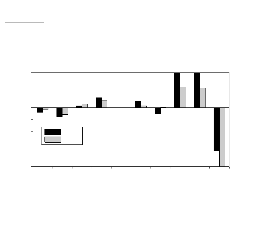
is assigned as PRE). If ∆P RE share < 0 we let ∆P RE share = 0 (i.e. none of a ﬁrm’s income

is assigned as PRE). Additionally, if net foreign income is negative and ∆PRE share < 0, we set

∆P RE share = 0.

We then measure how ﬁrms’ accumulation of PRE changed before and after 2003. We pick 2003

as this is the year in which the precursor bills leading up to the AJCA were ﬁrst introduced. We

do this by comparing a ﬁrm’s ∆P RE share by its average ∆P RE share from 1996-2002. This is

given by

∆P RE share

i,t

∆P RE share

i,t

∆P RE share

i,1996−2002

− 1

where ∆P RE share

i,1996−2002

is the ﬁrm’s average ∆P RE share from 1996-2002.

∆P RE share

i,t

gives the percentage point deviation of a ﬁrm’s accumulation of PRE as a share of foreign income

relative to its 1996-2002 average accumulation of PRE as a share of foreign income.

1996 1997 1998 1999 2000 2001 2002 2003 2004 2005

−1

−0.8

−0.6

−0.4

−0.2

0.2

0.4

0.6

Mean

Median

Figure A5:

∆P RE share 1996–2005

Notes: The ﬁgure shows the percentage point deviation of the share of foreign income retained abroad and un-

taxed by the US (PRE) relative to the average share from the period 1996–2002.

∆P RE share is deﬁned as

(∆P RE share)/(∆P RE share)

1996−2002

− 1 where ∆P RE share is the implied share of after tax foreign income

designated as PRE and ∆P RE share is the average ∆P RE share from 1996-2002.

Figure A5 plots the across-ﬁrm mean and median percentage point deviation of ∆P RE share

from its 1996-2002 average ∆P RE share,

∆P RE share. This gives a measure of how ﬁrms’

accumulation of PRE changed before versus after 2003, the year the precursor bills leading up to

the AJCA were ﬁrst introduced. Prior to 2003,

∆P RE share was relatively stable. From 2002-2003

and 2003-2004, this measure of changes in foreign asset holdings by U.S. ﬁrms increases sharply

relative to its long-run average. In 2004-2005,

∆P RE share substantially declined as ﬁrms ran

down their holdings of PRE by repatriating a large share of these assets during the tax holiday. We

note that the sharp increase in the accumulation of PRE in 2002-2003 occurred before the AJCA

was oﬃcially introduced and enacted. This is once again suggestive that ﬁrms anticipated the tax

holiday and acted on this anticipation by changing the amount of assets held overseas leading up

to the AJCA.

OA4 AJCA Literature and Model Comparison

In the early 2000’s policymakers were concerned that U.S. tax laws were disincentivizing U.S.

based multinationals from repatriating foreign income back to the U.S. They felt that if they

could convince ﬁrms to repatriate more foreign income it would lead to greater investment and

job creation in the U.S., thereby spurring further economic growth. Thus, in October 2004 they

passed the AJCA which reduced the maximum repatriation tax rate on qualiﬁed funds from 35

to 5.25 percent on 85 percent of repatriated earnings in a one-year window. Further, under the

AJCA guidelines, ﬁrms were required to use any funds that received tax breaks from the act on

U.S. employment, investment, research and development, and other uses related to job creation

and retention.

There is a large empirical literature that aims to tease out the eﬀects of the AJCA tax holiday on

a number of ﬁrm-level and ﬁscal policy variables. Table A1 summarizes the comparison between our

model ﬁndings and this empirical literature. The table shows our model is remarkably consistent

with the results documented in the empirical literature.

Table A1: AJCA Literature and Model Predictions

Study Period Study Findings Our Model Predictions

Transfers: Joint Committee on Taxation

(2004)

At/After Predicted transfers rise during the AJCA and fall after-

ward

Transfers rise during the tax holiday and

fall afterward.

U.S. Tax Revenue: Joint Committee

on Taxation (2004)

At/After An estimate of the budget impacts of the AJCA predicted

rise in tax revenue at the AJCA and fall thereafter for a

net loss in tax revenue.

Tax revenue rises during the tax holiday

and falls afterward for a net loss of U.S.

tax revenue.

Employment and Investment (Finan-

cially Unconstrained): Faulkender and

Petersen (2012), Dharmapala, Foley,

and Forbes (2011)

At/After No signiﬁcant change. Negligible total response.

Employment and Investment (Finan-

cially Constrained): Faulkender and Pe-

tersen (2012)

At/After Increase in investment and no change to employment. Increase in both variables (see Section 4.4

in main text).

Shareholder Payouts: Blouin and Krull

(2009), Dharmapala, Foley, and Forbes

(2011), Clemons and Kinney (2008)

At/After Increase in shareholder payouts (dividends and share re-

purchases). Dharmapala, Foley, and Forbes (2011) es-

timate a $1 increase in repatriation during the AJCA

correspond to a $0.60 to $0.92 increase in shareholder

payouts.

Increase in dividend payments approxi-

mately equaling the tax saving from hol-

iday.

Debt Reduction: Faulkender and Pe-

tersen (2012), Dharmapala, Foley,

and Forbes (2011), Graham, Hanlon,

Shevlin et al. (2010)

At/After Graham, Hanlon, Shevlin et al. (2010) ﬁnds ﬁrms with

foreign sourced earnings reported paying down domes-

tic debt as one of the most common uses of repatriated

earnings using survey data from tax executives from these

ﬁrms. The other papers ﬁnd no impact of the AJCA on

debt reduction.

Firms repay debt but the debt reduction is

short lasting.

Firm Value: Oler, Shevlin, and Wilson

(2007)

Pre Stock value increased proportionately to the expected tax

savings from the holiday. Increases occurred beginning

in 2003 when the passage of the AJCA seemed likely, but

the AJCA was not enacted until October 2004.

Increase in ﬁrm value V at the time of the

news of the tax holiday.

Notes: This table summarizes the impacts from the AJCA of 2004 from the literature and compares it with our model ﬁndings. The second column reports the sub-periods of the

analysis in the empirical literature in which the empirical studies focus on: Pre (news period) and At/After the enactment of the AJCA.

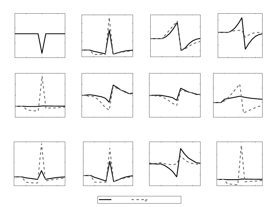
OA5 Sensitivity Analysis

OA5.1 Shareholder Preferences

In this section, we perform sensitivity analysis on the coeﬃcient of relative risk aversion σ in our

utility function. In our baseline simulation, we use log utility (σ = 1). Here we also show the case

when shareholders have risk neutral preferences (σ = 0).

-4 0 4

0.05

0.1

0.15

0.2

Repatriation tax rate

-4 0 4

200

400

600

800

Repatriations

-4 0 4

-100

100

200

Foreign financial assets

-4 0 4

-100

-50

U.S. debt

-4 0 4

-100

100

200

300

Dividends

-4 0 4

-1

-0.5

0.5

U.S. labor and capital

-4 0 4

-1

-0.5

0.5

U.S. output

-4 0 4

-2

Firm value (V)

-4 0 4

100

All sources

-4 0 4

200

400

Repatriations

-4 0 4

-1

-0.5

0.5

Corporate income

-4 0 4

100

200

300

Dividends

Baseline

=1 (linear utility)

Panel A: Firm-level responses

Panel B: US tax revenue by source

Figure A6: Responses to Temporary Reduction in Repatriation Taxes Where News of Reduction is

Received 4 Quarters in Advance

Notes: Except for the repatriation tax rate, units are in percent deviation from initial steady state. The ﬁgure plots the baseline

(σ = 1) and with risk neutral preferences (σ = 0).

Figure A6 shows the responses to news and the implementation of a tax holiday. The top

panel gives the ﬁrm-level responses and the bottom gives the responses for the U.S. government

tax revenue. The units are percentage deviations from the original stochastic steady state with the

exception of the repatriation tax rate graph which shows the actual time-path for the repatriation

tax rate. The tax holiday is implemented at period 0 and the ﬁrm receives news of it 4 quarters in

advance (period -4). The repatriation tax rate reduction is the same as in the baseline.

When we consider the case with linear utility, the results diﬀer quite substantially. Without

curvature in the utility of dividends, the ﬁrm does not have a motive to smooth out dividend

payments. Thus, there are wide swings in many variables at the announcement of the news. For

example, the ﬁrm cut oﬀ repatriations almost completely during the news period. The large swings

in foreign transfers, dividend payments, and U.S. tax revenue are at odds with the variation of

these variables for multinational ﬁrms in the data. In particular, with linear utility ﬁrms do not

have an incentive to smooth dividends over time. We thus, incorporate curvature in out utility

function.

OA5.2 Foreign Borrowing

Here we relax the restriction that foreign operations cannot access external credit markets and allow

them to borrow as they can domestically. The ﬁrm therefore faces a worldwide interest rate on

borrowing – i.e. the interest rate on debt is the same across both jurisdictions. Figure A7 shows the

model results from the baseline exercise (no foreign borrowing) and with foreign borrowing. The

top panel gives the ﬁrm-level responses and the bottom gives the responses for the U.S. government

tax revenue. The units are percentage deviations from the original stochastic steady state, with the

exception of the repatriation tax rate graph, which shows the actual time-path for the repatriation

tax rate. The tax holiday is implemented at period 0 and the ﬁrm receives news of it 4 quarters in

advance (period -4). The repatriation tax rate reduction is the same as in the baseline.

When there is foreign borrowing, increases in foreign ﬁnancial asset holdings rise much more

sharply than in the baseline during the news period. However, we note that although the percentage

change is larger, the steady state level of foreign asset holdings is smaller than in the baseline. In

fact, a large part of the transferred assets during the tax holiday when there is foreign borrowing

comes from assets used to ﬁnance production abroad. Immediately after the transfer, foreign

operations overcome this shortcoming with a rapid increase in foreign debt.

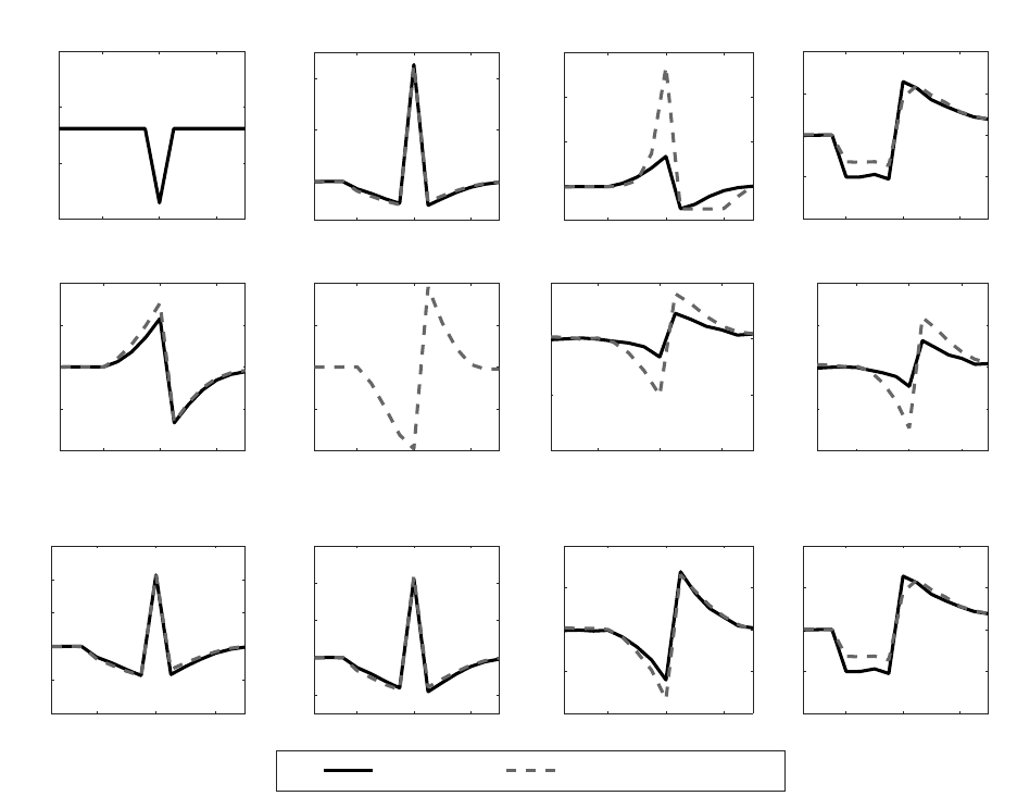
-4 0 4

0.05

0.1

0.15

0.2

Repatriation tax rate

-4 0 4

200

400

Repatriations

-4 0 4

200

400

600

Foreign financial assets

-4 0 4

-4

-2

Dividends

-4 0 4

-100

-50

100

U.S. debt

-4 0 4

-100

-50

100

Foreign Debt

-4 0 4

-2

-1

U.S. labor and capital

-4 0 4

-1

-0.5

0.5

U.S. output

-4 0 4

-20

-10

All sources

-4 0 4

-100

100

200

300

Repatriations

-4 0 4

-1

-0.5

0.5

Corporate income

-4 0 4

-4

-2

Dividends

Baseline with foreign borrowing

Panel A: Firm-level responses

Panel B: US tax revenue by source

Figure A7: Responses to Temporary Reduction in Repatriation Taxes Where News of Reduction is

Received 4 Quarters in Advance when Firms can Borrow both in the U.S. and Abroad.

OA5.3 Permanent Repatriation Tax Cut

Here we consider the case when the repatriation tax changes is implemented as a permanent reduc-

tion. Figure A8 shows the transition graph for the case of a permanent reduction in repatriation

tax rates. The ﬁrm unexpectedly receives a tax news shock that notiﬁes them there will be a

permanent tax policy change T quarters in the future. Once the tax reform is implemented, the

tax rate remains at this new level indeﬁnitely.

…

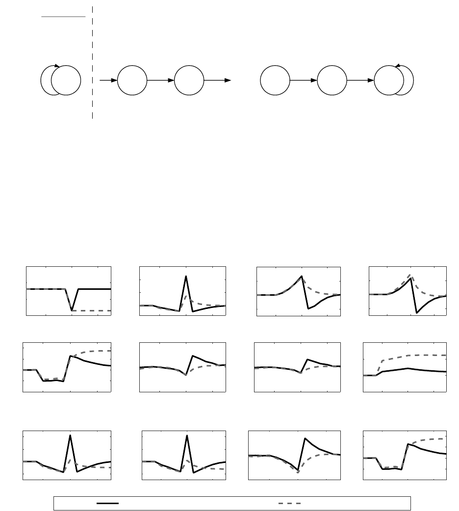
Steady State

Tax

News

Tax

Reform

Prob = 1

Period 1 Period 2

Steady

State

Prob = 1 Prob = 1 Prob = 1 Prob = 1

Period T–2

Period T–1

Figure A8: Transition Graph Where a Permanent Change in Tax Policy Occurs T Periods

From Arrival of the News

Figure A9 shows the responses to a permanent repatriation tax reduction announced 4 periods

in advance plotted alongside the baseline results for comparison. The size of the repatriation tax

reduction is the same as in the baseline.

-4 0 4

0.05

0.1

0.15

Repatriation tax rate

-4 0 4

200

400

600

Repatriations

-4 0 4

-100

100

200

Foreign financial assets

-4 0 4

-50

100

U.S. debt

-4 0 4

-4

-2

Dividends

-4 0 4

-1

U.S. labor and capital

-4 0 4

-1

U.S. output

-4 0 4

-2

Firm value (V)

-4 0 4

-10

All sources

-4 0 4

-100

100

200

Repatriations

-4 0 4

-1

Corporate income

-4 0 4

-4

-2

Dividends

Temporary tax cut (Baseline) Permanent tax cut

Panel A: Firm-level responses

Panel B: US tax revenue by source

Figure A9: Responses to a permanent reduction in the repatriation tax rate were news of reduction is

received 4 Quarters in Advance. Units are in percent deviation from initial steady state.

In the news period, ﬁrms reduce transfers at approximately the same rate as the baseline. At

the policy change, the ﬁrm repatriates the assets accumulated during the news period, but the total

amount repatriated in this period is less than the baseline. When the tax change is temporary,

ﬁrms have incentive to shift foreign income that would otherwise be transferred in future periods

to exploit the one-time tax saving on these assets. When the change is permanent, ﬁrms have

no such motive since these repatriated assets will indeﬁnitely face a lower tax rate. This is why

repatriations at the time of the policy change is less responsive for a permanent than a temporary

tax reduction.

After the permanent repatriation tax reduction, U.S. output and capital and labor use is per-

manently higher in the steady state, albeit is very small (approximately 1/20 of 1 percent). Addi-

tionally, the permanent tax rate reduction leads to a perpetual loss to U.S. tax revenues: a lower

tax rate yields lower tax revenues. In sum, gains to U.S. output and factor input use is small and

U.S. tax revenue losses are large from this permanent repatriation tax reduction. In comparison,

Arena and Kutner (2015) study the empirical impacts of permanent repatriation tax reductions

from the 2009 reforms in Japan and the United Kingdom. They do not ﬁnd evidence of increases

in domestic investment. Again, in our model domestic capital use increases by 1/20 of 1 percent.

OA5.4 Discussion On General Equilibrium

For the case of a permanent reduction in repatriation tax rates, we believe our framework is

informative to understand the dynamics around a local period from the time of the news period

to after the policy change. In the long run, however, there may general equilibrium eﬀects from a

permanent repatriation tax change that we do not capture as ﬁrms and households adjust to a new

tax environment.

Our model, for one, does not capture the additional production – and the subsequent eﬀects –

that could emerge from eﬃciency gains following a reduction in distortionary taxes. From a tax

revenue perspective, this would imply that when the repatriation tax rates are lower, the taxable

base may be larger. If the eﬃciency gains are large enough, it could be that tax revenue does not

decrease much during the announcement and after the holiday. At the ﬁrm level, the substitution

eﬀect from the reduction in taxes on repatriations – or its announcements – may remain unchanged:

taxes in the present became relatively higher. The income eﬀect, however, would be heighten as

the value of the ﬁrm increases. The latter would dampen the reduction in dividend payments in

the news period. Depending on the level of dividends, it could be that the marginal increases are

See, for example, Spencer (2017) for a general equilibrium model of permanent repatriation tax rate changes.

devoted to production during the time of the announcement which could imply that, even if ﬁrms

are ﬁnancially constrained, labor and capital does not contract.

Second–as mentioned in the main text in more detail – as ﬁrms adjust their demand for inputs

in response to the policy change, input prices would respond accordingly. Most likely, these price

adjustments in factor inputs would also serve to dampen the responses to labor/capital and output

in comparison to the relatively small responses in our baseline model. As the asset ﬂows into the

U.S. in response to the tax reduction, this would make consumers wealthier – from an inﬂux of

dividends and/or higher factor payments – and result in an increase in demand for goods and

services from the ﬁrms.

In both cases – eﬃciency gains and price changes – the income eﬀect would be larger and there

would be no substitution eﬀect of tax rates (i.e. in the case of an announcement, future repatriation

tax rates became cheaper). These would arguably dampen the responses we ﬁnd at the ﬁrm level.

The response of labor would hence depend on the extent to which wealth eﬀects are assumed in

the household’s preferences. What is clear, however, is that the aggregate and welfare eﬀects of

repatriation taxes would necessitate a general equilibrium to be properly quantitatively evaluated

in the case of permanent changes in repatriation taxes. Our framework, nevertheless, highlights

important mechanisms at the ﬁrm level that are consistent with the empirical literature and that

such a framework should capture.

OA6 Tax Cut and Jobs Act of 2017

Here, we use our framework to analyze the periods leading up to, and implementation of, the

most recent tax reforms: the Tax Cut and Jobs Act of 2017 (henceforth the TCJA17 to clearly

distinguish the acronym from the AJCA). The TCJA17 includes comprehensive tax reforms that

include, but are not exclusive to, changes in the taxation of foreign activity of U.S. multinationals.

Our analysis strictly focuses on the aspects that impact the taxation of multinationals.

Calls for changes in the taxation of U.S. based multinationals were continuously proposed by

both Democrats and Republicans in the years leading up to the TCJA17. This included President

Obama’s White House Budgets for 2015, 2016, and 2017, and The Blueprint – a leading Republican

tax reform plan introduced in the House of Representatives in 2016. Expectations of a heightened

possibility of tax reform took hold after the elections of 2016 which aligned Republican majorities

in both houses of congress and in the presidency. President Trump’s administration unveiled their

outline for tax reform in April 2017 where Treasury Secretary Mnuchin stated that they would

move as fast as they can on passage and implementation. The TCJA17 was brought to congress

later that year was signed into law on December 2017 and went into eﬀect at the beginning of 2018.

The act reduced U.S. corporate income tax from a top marginal tax rate of 35% to a ﬂat tax of

21%. Second, the TCJA17 moved the U.S. to a territorial tax system – a 100 percent tax exemption

on all income generated abroad by U.S. multinationals, i.e. an elimination of repatriation taxes.

Finally, it implemented a one-time “deemed repatriation tax” bridging the former international tax

regime to a new one. This is a one-time retroactive tax on the sum of foreign income held abroad

that was untaxed by the U.S. government at the time of the implementation date. Following this

one-time tax, these assets were able to be repatriated with no additional U.S. tax costs.

Within our model, we can implement the changes of the TCJA17. Letting the date of imple-

mentation be time t = J, U.S. corporate income taxes in the model are given by

= 0.302 if t < J (OA6.1)

= 0.21 if t ≥ J. (OA6.2)

The model repatriation tax rate is similarly given as

τ = 0.131 if t < J (OA6.3)

τ = 0.0 if t ≥ J. (OA6.4)

Under the TCJA17, the deemed repatriation tax applies to all foreign assets yet to be taxed by

the U.S. government and accumulated since the enactment of the Tax Reform Act of 1986. In the

model, the transition tax is applied to all foreign assets, A

, at the period of the tax reform minus

the initial transfer from the U.S. parent to set up the foreign operation. Assuming the foreign

operation was established at time t = 0 and the tax reform is initiated at time t = J, then the

assets facing the transition tax is

F,J

− T

t=0

F,t

(1 − τ

) −

t=1

where T

is the initial transfer from the ﬁrm’s U.S. operations and π

are the sum of pre-tax

foreign income from operations and interest on bank assets. In the model, we assume the seed

money from the U.S., T

, is small relative to the total assets at time T . Thus, tax revenues from

the transition tax τ

T T

is τ

T T

F,T

. The TCJA levies the deemed repatriation tax rate of 15.5%

on cash and cash equivalents (liquid assets) and 8% on remaining assets. Given the fungibility of

internal funds, in our model the diﬀerential taxation on liquid vs. non-liquid assets is problematic

as ﬁrms can immediately change the composition of asset holdings – particularly if the tax change

is anticipated. For this reason, we impose the transition tax to be τ

T T

= 0.104 which is calculated

by weighting the two tax rates by the relative shares of liquid and non-liquid assets to total foreign

assets in the model steady state.

In this exercise, the ﬁrm knows with certainty that the TCJA17 will occur 4 periods in advance

of its implementation. This corresponds with a news period over the 2017 calendar year with

implementation in 2018Q1. The solid lines in Figure A10 present the responses to news of and

implementation of the provisions in the TCJA17. We additionally include a simulation with all of

the tax changes in the TCJA17 except the deemed repatriation tax (dashed line) to highlight the

role deemed repatriation taxes play on the dynamics. We note that although from the Figure it is

clear the dynamics diﬀer, both simulations eventually converge to the same steady state.

During the news period, ﬁrms that face the deemed repatriation tax withhold fewer repatriations

and accumulate less foreign ﬁnancial assets as this tax reduces the incentives for ﬁrms to accumulate

assets abroad. From a policy perspective, if lawmakers wanted to draft a tax policy change that

mitigates the incentives for ﬁrms to accumulate foreign assets in expectation of tax reform, including

a deemed repatriation tax is a better option in this dimension than just purely permanently changing

the tax rates. The size of the deemed repatriation tax, however, still results in tax gains for the

ﬁrm.

In the short run, the TCJA17 leads to short run losses in labor/capital and output before and in

the periods after the policy change. The deemed repatriation tax drives this result because this tax

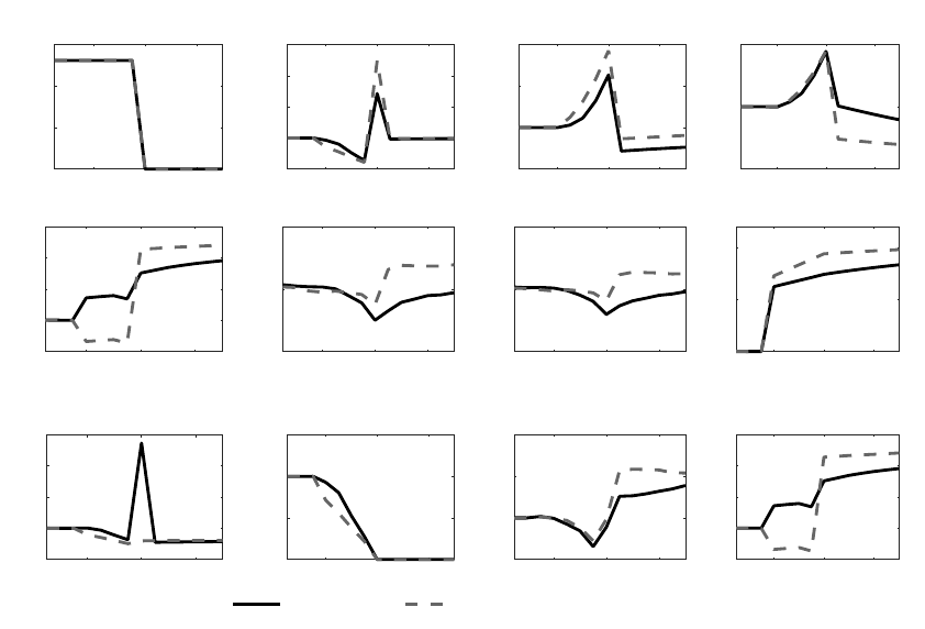
removes a portion of the ﬁrm’s stock of assets and, since the cost of debt is a function of its assets,

higher borrowing cost reduce the ﬁrm’s ability to ﬁnance production with debt. However, if the

timeline were extended we would see that in the ﬁnal steady state labor/capital are just 1/2 percent

larger than before the policy change. At the time of the policy change, U.S. tax revenues spike

from the one-time deemed repatriation tax. All of the tax revenue losses after the enactment period

come solely from reductions in repatriation tax receipts. In the short run, the deemed repatriation

tax results in sizable tax revenues for the U.S. government.

-4 0 4

0.05

0.1

0.15

Repatriation tax rate

-4 0 4

-100

100

200

300

Repatriations

-4 0 4

-100

100

200

Foreign financial assets

-4 0 4

-50

U.S. debt

-4 0 4

-5

Dividends

-4 0 4

-1

U.S. labor and capital

-4 0 4

-1

U.S. output

-4 0 4

Firm value (V)

-4 0 4

-20

All sources

-4 0 4

-100

-50

Repatriations

-4 0 4

-0.5

0.5

Corporate income

-4 0 4

-5

Dividends

TCJA17 TCJA17 without deemed repat. tax

Panel A: Firm-level responses

Panel B: US tax revenue by source

Figure A10: Response to News and Implementation of the Tax Cut and Jobs Act of 2017

Notes: Firms receive news of the TCJA17 4 quarters in advance. The policy change includes a deemed repatriation

tax of 10.4 percent at the time of the policy change only, and permanent reductions of U.S. corporate income tax

rate to 21% and a removal of repatriation taxes (τ

= 0). The solid line has all of the policy changes and the

dashed line has all of the policy changes except the deemed repatriation tax.

OA References

Arena, M. P. and G. W. Kutner (2015): “Territorial Tax System Reform and Corporate

Financial Policies,” Review of Financial Studies, hhv005.

Blouin, J. and L. Krull (2009): “Bringing it Home: A Study of the Incentives Surrounding the

Repatriation of Foreign Earnings Under the American Jobs Creation Act of 2004,” Journal of

Accounting Research, 47, 1027–1059.

Clemons, R. and M. Kinney (2008): “An Analysis of the Tax Holiday for Repatriation Under

the Jobs Act,” Tax Notes, 120.

Dharmapala, D., C. F. Foley, and K. J. Forbes (2011): “Watch What I do, Not What I

Say: The Unintended Consequences of the Homeland Investment Act,” The Journal of Finance,

66, 753–787.

Faulkender, M. and M. Petersen (2012): “Investment and Capital Constraints: Repatriations

Under the American Jobs Creation Act,” Review of Financial Studies, 25, 3351–3388.

Foley, C. F., J. C. Hartzell, S. Titman, and G. Twite (2007): “Why Do Firms Hold So

Much Cash? A Tax-Based Explanation,” Journal of Financial Economics, 86, 579–607.

Graham, J. R., M. Hanlon, T. Shevlin, et al. (2010): “Barriers To Mobility: The Lockout

Eﬀect Of US Taxation Of Worldwide Corporate Proﬁts,” National Tax Journal, 63, 1111–1144.

Joint Committee on Taxation (2004): “Estimated Budget Eﬀets of the Conference Agreement

for H.R. 4520, The ‘American Jobs Creation Act of 2004’,” JCX-69-04, Joint Committee on

Taxation, Washington D.C.

Oler, M., T. Shevlin, and R. Wilson (2007): “Examining Investor Expectations Concerning

Tax Savings on the Repatriations of Foreign Earnings Under the American Jobs Creation Act of

2004,” Journal of the American Taxation Association, 29, 25–55.

Spencer, A. (2017): “Policy eﬀects of international taxation on ﬁrm dynamics and capital struc-

ture,” Working Paper.