
BLM 2021
2020 BLM Specialist Report on Annual
Greenhouse Gas Emissions
and Climate Trends
from Coal, Oil, and Gas Exploration and Development on the
Federal Mineral Estate

BLM 2021
Page
3
7
10
17
21
38
56
64
72
86
100
106
109
113
Table of Contents
Executive Summary
1.0 Introduction
2.0 Relationships to Other Laws and Policies
3.0 Greenhouse Gases
4.0 Methods and Assumptions
5.0 GHG Emissions and Projections from BLM-Authorized Actions
6.0 Global, National, and State GHG Emissions
7.0 Emissions Analysis
8.0 Climate Change Science and Trends
9.0 Projected Climate Change
10.0 Mitigation
Glossary of Terms
References
Annex

BLM 2021
The "
2020 BLM Specialist Report on Annual Greenhouse Gas Emissions and Climate Trends
" presents the
estimated emissions of greenhouse gases (GHGs) attributable to fossil fuels produced on lands and mineral
estate managed by the Bureau of Land Management (BLM). More specifically, this report is focused on
estimating GHG emissions from coal, oil, and gas development that is occurring, and is projected to occur, on
the federal onshore mineral estate. The report includes a summary of emissions estimates from reasonably
foreseeable federal fossil fuel development and production over the next 12 months, as well as longer term
assessments of potential federal fossil fuel GHG emissions and the anticipated climate change impacts
resulting from the cumulative global GHG burden. The report is an important tool for evaluating the
cumulative impacts of GHG emissions from fossil fuel energy leasing and development authorizations on the
federal onshore mineral estate relative to several emission scopes and base years.
Emissions estimates were developed using fiscal year (FY) 2020 data for both direct and indirect emissions.
can result from authorized activities such as drilling or venting, while
occur as a consequence of the authorized action and can include activities such as the processing,
transportation, and any end-use combustion of the fossil fuel mineral products. The emission estimates are
expressed as (Mt) of carbon dioxide equivalents (CO e) on either a rate or absolute basis. Table
ES-1 shows the estimated GHG emissions from from the Federal mineral estate
in FY 2020. Table ES-2 shows the 2020 emissions by state, where extraction is the direct portion of the
emissions, and processing and transport represent a portion of the indirect emissions along with the end-use
estimates.
Table ES-1. Estimated Annual GHG Emissions from Existing Federal Fossil Fuel
Production in 2020 (Mt CO e)
2020 annual emissions based on fiscal year production data (i.e., Oct. 1 - Sept. 30)
Direct emissions indirect emissions
megatonnes
2
actual fossil fuel production
2
BLM Authorized Development Direct Indirect End Use Total
Coal 4.85 27.36 458.74 490.95
Oil 25.00 18.08 136.36 179.44
Gas 20.44 50.51 177.29 248.24
Total 2020 Existing 50.3 95.9 772.4 918.6
Executive Summary

BLM 2021
Table ES-2. Estimated Annual Federal Emissions by State - 2020 (Mt CO e)
Table ES-3 provides an estimate of (1) present emissions from existing production that is anticipated to keep
producing and (2) reasonably foreseeable future GHG emissions, including (a) emissions from previously
authorized development that is not currently producing but may begin production and (b) potential new
leasing that could begin producing. This table also provides estimated cumulative GHG emissions over the
typical production life for existing and new development projected to occur over the next fiscal year. The
typical production life for an oil and gas well can vary considerably based on multiple factors but generally
ranges from 20 to 25 years. The projected emissions estimates generated in this report are based on a
conservative assumption that the production life for new oil and gas wells is 30 years (with decline). The
2
50.2766 21.505 74.4534 772.39 918.62
14.5008 4.7627 41.0384 452.84 513.14
23.3699 11.6466 17.25 151.47 203.74
4.7509 1.4989 8.4371 62.58 77.27
1.6932 0.5833 2.4352 40.91 45.62
3.6897 2.0294 1.8776 26.88 34.48
0.4949 0.1584 1.7523 25.59 28
0.7979 0.464 0.1869 4.49 5.94
0.2064 0.0765 0.3712 1.68 2.33
0.1873 0.0812 0.2495 1.38 1.9
0.1553 0.0564 0.2883 1.27 1.77
0.1619 0.0588 0.2003 1.21 1.63
0.1022 0.0194 0.1255 0.83 1.08
0.051 0.0165 0.1095 0.44 0.62
0.0281 0.0113 0.044 0.21 0.29
0.0233 0.0077 0.0487 0.2 0.28
0.0198 0.0115 0.0053 0.11 0.14
0.019 0.0112 0.0025 0.1 0.13
0.0126 0.0063 0.0113 0.08 0.11
0.0077 0.0027 0.0148 0.06 0.08
0.0007 0.0002 0.0016 0.01 0.01
0.0015 0.0009 0.0002 0.01 0.01
0.0009 0.0004 0.0013 0.01 0.01
0.0004 0.0001 0.0008 0 0
0.0003 0.0001 0.0007 0 0
0 0 0.0001 0 0
0.0007 0.0004 0.0001 0 0
0.0001 0 0.0002 0 0
Extraction CO2e Processing CO2e Transport CO2e Combustion CO2e Total CO2e
Federal Total
WY
NM
CO
UT
ND
MT
CA
LA
AK
TX
OK
AL
AR
KS
OH
MS
NV
SD
MI
VA
NE
KY
WV
PA
NY
IL
ID
Area

BLM 2021
typical production life assumed for coal production is 1 year as most coal is typically produced and
consumed in a single year. The annualized emissions rates shown in Table ES-3 are a subset of the life-of-
project emissions data, specifically the emissions from year one (i.e., the next 12 months).
Table ES-3. Estimated GHG Emissions from Reasonably Foreseeable Projected Federal Fossil Fuel
Production over the Next 12 Months
Emissions are based on life-cycle-assessment (LCA) data factors that are relative to total production and include non-
combusted GHGs (e.g., fugitive CH ).
Indirect emissions include LCA values for transportation/distribution, processing/refining, but NOT end use
(combustion), which is shown separately for illustrative purposes.
Direct and Indirect emissions are additive for life-cycle accounting but represent a double count for annual reporting.
Life-of-Project emissions for Oil and Gas are a 30-year declined-projection for each authorization type shown. Coal
emissions are based on a single year of forecasted production (see coal discussion in Chapter 4.2).
Table ES-4 provides the long-term cumulative sums of production, energy values, and GHG emissions
projected out to year 2050 based on data obtained from the U.S. Energy Information Administration's Annual
Energy Outlook 2021 report. The projections are made by multiplying each year of data from the AEO report
by the most current 5-year averages of federal production divided by the 5-year averages of total U.S.
production for each fossil fuel mineral type.
BLM Authorized Development Mt CO2e/yr (Annual) Mt CO2e (Cumulative)
Direct Indirect End Use Totals Life-of-Project
Existing Federal Production
Coal 5.66 30.47 509.92 546.05 546.05
Oil 18.97 13.73 103.48 136.18 1,062.08
Gas 16.53 40.86 143.40 200.79 2,074.62
Subtotal Existing Production 41.2 85.1 756.8 883.0 3,682.7
Permitted but NOT yet developed Oil, Gas, and Coal Leases
Coal 0 0 0 0 0
Oil 24.04 17.39 131.18 172.61 366.42
Gas 7.11 17.56 61.70 86.37 289.77
Subtotal Approved Permits 31.2 35.0 192.9 259.0 656.2
Potential New Leases
Coal 0 0 0 0 0
Oil 10.20 7.38 55.62 73.09 192.57
Gas 6.07 15.00 52.65 73.72 322.05
Subtotal Potential 16.3 22.4 108.2 146.8 514.6
Total Projected Emissions over the next 12 Months
Coal 5.66 30.47 509.92 546.05 546.05
Oil 53.19 38.49 290.20 381.88 1,621.07
Gas 29.71 73.42 257.75 360.88 2,686.44
Total CO2e 88.6 142.4 1,057.9 1,288.8 4,853.6
4

BLM 2021
Table ES-4. Long-Term (2021 - 2050) Onshore Federal Mineral Projections
5-year average ratio of fossil fuel historical production data equals federal (ONRR) / U.S. Totals (EIA).
AEO Reference Case used for series projections, and totals are the sum of the series (2021 - 2050).
Additional details on emissions estimation methodologies and calculation results are presented in Chapters
4 and 5. Chapters 1 through 3 provide background information on the purpose of this document, applicable
laws, and the GHGs of interest to the BLM. The remainder of the document (Chapters 6 through 10) provides
comparative context for the estimated emissions, the impacts of climate change, and potential mitigation
strategies.
* * *
Federal Minerals Production Energy (Quads) Emissions (Mt CO e)
2
Coal (MM short tons) 5,325.36 132.7612 10,151.36
Oil (MM b/d) 24.43 51.6835 5,089.09
Gas (Tcf) 117.71 119.2700 8,871.90
Projected Totals NA 303.71 24,112.35

BLM 2021
1.1 Purpose
The "
2020 BLM Specialist Report on Annual Greenhouse Gas Emissions and Climate Trends
" provides a
detailed assessment of greenhouse gas (GHG) emission trends and potential climate impacts from energy
development projects, specifically those that may result from the Bureau of Land Management (BLM)
authorized coal, oil, and gas and approved development on (including the federal mineral
estate) managed by the BLM. This report examines carbon emissions from authorized development of the
onshore in the context of the nation's carbon economy and the relationship between
energy generation and climate issues by providing life-cycle estimates of fossil fuel greenhouse gas
emissions from that development. The report provides estimates of both direct and indirect emissions from
development and consumption of onshore federal fossil fuel minerals, including those fuels that are
combusted by end users (when off-lease). This report incorporates current climate science and discussions
of scientific values relevant to the context within which the BLM authorizes development of the onshore
federal mineral estate. This report is designed to be updated on an annual basis and serves as a tool to track
the evolution of climate science and policy inorder to provide decision makers with the best available data to
implement management strategies consistent with regulatory requirements.
1.2 Background
Coal, oil, and gas are examples of fossil fuels found in the Earth’s crust that formed from decomposing
plants and animals. These fuels contain high concentrations of carbon and hydrogen that can be burned for
energy. The extraction, production, and consumption of these fossil fuels produce GHGs, particularly carbon
dioxide and methane, which in turn trap heat in the atmosphere causing the “greenhouse effect”, resulting in
an increase in average global temperatures and other climatic changes over time. The BLM’s authorization of
fossil fuel energy development can result in both direct and indirect emissions of GHGs that contribute to
global climate change. Direct emissions can result from authorized activities such as drilling or venting,
while indirect emissions occur as a consequence of the authorized action and can include activities such as
the processing, transportation, and any end-use combustion of the fossil fuel mineral products.
As the steward of the greatest percentage of , the BLM manages about 245 million acres of
public lands encompassing approximately 10 percent of the nation’s total surface area. In addition, the BLM
administers the onshore federal mineral estate (subsurface) which covers a total of about 710 million acres
from the eastern United States to Alaska (BLM 2020) . In keeping with its
mandate prescribed in accordance with the Federal Land Policy and Management Act (FLPMA) of 1976 and
the Mineral Leasing Act (MLA) of 1920 (30 U.S.C. 181 et seq.), the BLM leases minerals including coal, oil,
and gas on the onshore federal mineral estate and authorizes development of these leased minerals.
Approximately 26.4 million acres of the federal mineral estate have been leased through BLM’s coal leasing
and oil and gas leasing programs. Slightly less than half (approximately 48%, or 13 million acres) of the
leased mineral estate are currently producing federal fossil fuels (coal, oil, gas). Statistics maintained by the
Office of Natural Resources Revenue (ONRR) show that approximately 246 million tons of coal, 314 million
barrels of oil and 3.3 billion cubic feet of gas were produced from these 13 million acres in 2020, or about
46% of the nation's coal supply, and 7.6% and 9.1% of the nation's oil and gas supply, respectively. Note: The
leases public lands
federal mineral estate
federal lands
[1]
multiple use and sustained yield
1.0 Introduction

BLM 2021
total area of onshore federal mineral estate does not imply that economically recoverable quantities of
minerals exist at that scale; it is simply an administrative area.
1.3 Using this Report
Consistent with 40 C.F.R. § 1501.12 (Incorporation by reference) and mandates to reduce paperwork,
National Environmental Policy Act (NEPA) document preparation time, and overall NEPA document lengths,
this report may be incorporated by reference (IBR) into applicable NEPA documents to aid in describing
reasonably foreseeable environmental trends in the affected environment (40 CFR § 1502.15), and to provide
context for impacts analysis of GHG emissions resulting from the federal action being analyzed. Consistent
with the Council on Environmental Quality (CEQ), Department of the Interior regulations and BLM policy, when
this report is incorporated by reference, the BLM must cite and summarize this report (see 40 CFR § 1501.12;
43 CFR § 46.135; and BLM Handbook H-1790-1, "NEPA Handbook", chapter 5.2.1) and ensure it is available
for inspection by potentially interested persons. In the course of incorporating this report by reference, the
NEPA document should also explicitly incorporate all linked content and reference materials used in this
report to provide for a complete record. Note: This report does not take the place of an analysis and
disclosure of emissions at the project level that may be completed for NEPA analysis specific to a decision to
lease or authorize development, but this report supplements that analysis by providing an evaluation of
cumulative emissions from fossil fuel authorizations on a state and national level.
This report is available in two formats: a static report and a dynamic online tool. The static version is
essentially any printed version of the dynamic web tool, and should be used to support the administrative
records for applicable federal decisions at the point in time that NEPA analysis is conducted. The web-based
version is dynamic and allows for real-time data incorporation and transformations that are not easily
replicated in a nondigital format. The web version is built to be interactive and allow readers to quickly
explore and find various datasets such that the context and conclusions of the report can be easily
understood. Dynamic content contained within the various report elements will load and render applicable
datasets based on the user's interaction with the element's control(s). The interactive design means that
readers will need to take care to ensure that any dynamic datasets of interest are rendered (i.e., visible) in the
document prior to printing the report, as the browser will only print what is rendered. For example, most of
the charts in this report allow users to explore multiple datasets, however only the visible dataset is printed.
The report will not print all of the available chart configurations for a particular dataset which could number
in the hundreds. Users can save individual charts by right clicking and selecting "save image as..." to
download a copy, and in most case the data for a rendered chart can be downloaded as well.
This report was prepared by air quality, fluid minerals, and leasing specialists across the BLM, to make a
broad but concerted effort to utilize and present the best data and statistics available for estimating
emissions associated with BLM-authorized actions in a consistent manner. This data was analyzed using the
best available science applicable to the onshore federal mineral estate. As new information and models
become available, the BLM will continue to improve and revise its emission estimates, methodologies, and
assumptions as appropriate. This report will be updated annually, and each annual version of the report will
review the accuracy of the estimates and projections represented in previous versions and will incorporate
actual data from the previous year, to calibrate assumptions used in the next year’s emissions estimates and
projections and thereby improve the accuracy of each iteration of the report.

BLM 2021
1.4 Disclaimer
Much of the sourced information for this report has been obtained, summarized, or linked from the
presentations of various governmental agencies, international institutions, and nongovernmental
organizations. All information in this report is being provided "as is", and while the authors made every
attempt to ensure that the information is timely, complete, accurate, and obtained from reliable sources, the
BLM makes no guarantee that it is free of errors or omissions. Hyperlinks contained within the report
connect to other websites that are maintained by other Federal Government agencies or nonfederal entities
over which the BLM exercises no control. The BLM does not make any representation as to the accuracy or
any other aspect of information contained in linked content or data obtained from external application
programming interfaces. The projections and evaluations of the data developed and disclosed in this report
are presented strictly to display assumptions for analysis and should not be interpreted as an exacting
prediction or guarantee of future conditions, emission trends, or as an emissions cap or authorization limit.
This report is not intended to, and does not create any right or benefit, substantive or procedural, enforceable
at law or in equity by a party against the United States, its departments, agencies, or entities, its officers,
employees, agents, or any other person.
* * *

BLM 2021
2.1 Federal Land Policy and Management Act
The Federal Land Policy and Management Act (FLPMA) of 1976 (43 U.S.C. §§ 1701-1785), provides the
majority of the BLM’s legislated authority, policy direction, and basic management guidance. This act
outlines the BLM’s role as a multiple use land management agency and provides for management of the
public lands under principles of multiple use and sustained yield unless otherwise provided by law. The act
states a policy that public lands are to be managed “in a manner that will protect the quality of scientific,
scenic, historical, ecological, environmental, air and atmospheric, water resource, and archeological values”
(Sec. 102(a)(8)). To fulfill this responsibility, the BLM's land use plans ensure “compliance with applicable
pollution control laws, including State and Federal air, water, noise, or other pollution standards or
implementation plans” (Sec. 202(c)(8)). Accordingly, BLMs leases and operating permits for fossil fuels
require compliance with all state and federal air pollution requirements. FLPMA also gives the BLM authority
to revoke or suspend any BLM-authorized activity that is found to be in violation of regulations applicable to
public lands and/or noncompliance with applicable state or federal air quality standards or implementation
plans, thus ensuring that the BLM can provide for compliance with applicable air quality standards,
regulations, and implementation plans (Sec. 302(c)). Thus, for purposes of analysis, the BLM assumes full
compliance with applicable state and federal air quality requirements, emissions standards, and related
equipment and performance standards in effect at the time of the writing of the report.
2.2 Mineral Leasing Act
The Mineral Leasing Act of 1920, (MLA) as amended (30 U.S.C. 181 et seq.) authorizes and governs leasing
of public lands for development of deposits of coal, oil, gas and other hydrocarbons, sulphur, phosphate,
potassium and sodium. Section 185 of this title contains provisions relating to granting of rights-of-ways
over Federal lands for pipelines. The MLA and the Mineral Leasing Act for Acquired Lands of 1947 give the
BLM responsibility for oil and gas leasing of minerals underlying about 700 million acres of BLM-managed
surface lands, National Forest System lands, other Federal lands managed by other agencies, and State and
private surface lands where the mineral rights underneath were retained by the Federal government. The
Federal Onshore Oil and Gas Leasing Reform Act of 1987 (Sec. 5102) amended the MLA (30 USC 226), and
directs the BLM to conduct lease sales for each State where eligible lands are available at least quarterly.
Leases are first offered for sale at competitive auctions and then are made available non-competitively, for
two years, if a qualified bid is not received at the competitive sale.
2.3 National Environmental Policy Act
The National Environmental Policy Act (NEPA) of 1969 (42 U.S.C. § 4321 et seq.) ensures that information on
the potential environmental and human impact of federal actions is available to public officials and citizens
before decisions are made and before actions are taken. One of the purposes of the act is to “promote
efforts which will prevent or eliminate damage to the environment and biosphere,” and to promote human
health and welfare (Section 2). This act requires that agencies prepare a detailed statement on the
environmental impact of the proposed action for major federal actions expected to significantly affect the
quality of the human environment (Section 102(C)). In addition, agencies are required, to the fullest extent
possible, to use a “systematic, interdisciplinary approach” in planning and decisionmaking processes that
may have an impact on the environment (Section 102(A)).
2.0 Relationships to Other Laws and Policies

BLM 2021
2.4 Council on Environmental Quality
The Council on Environmental Quality (CEQ) is an entity within the executive office of the President that is
responsible for coordinating federal efforts to improve, preserve, and protect America’s public health and
environment. The CEQ oversees the implementation of NEPA by issuing guidance, interpreting regulations,
and approving federal agency NEPA procedures.
The CEQ issued final guidance for federal agencies on analyzing GHGs in NEPA documents in 2016 ("Final
Guidance for Federal Departments and Agencies on Consideration of Greenhouse Gas Emissions and the
Effects of Climate Change in National Environmental Policy Act Reviews"). The CEQ rescinded that guidance
in 2017 and released new draft guidance in 2019. On February 19, 2021, pursuant to Executive Order 13990,
"Protecting Public Health and the Environment and Restoring Science to Tackle the Climate Crisis", the CEQ
rescinded the 2019 draft NEPA guidance on consideration of GHGs and is reviewing, for revision and update,
the previously recinded 2016 final guidance. In the interim, the CEQ has advised federal agencies to consider
all available tools and resources in assessing GHG emissions and climate change effects of their proposed
actions, including the previously rescinded 2016 GHG guidance.
2.5 Executive Orders
Executive orders (EOs) and memoranda issued in 2021 address the climate crisis and focus on GHG
emission reductions and increased renewable energy production. The orders rescind previous CEQ guidance
on analysis of GHG emissions, with the goal of reviewing, revising/updating, and issuing new guidance on the
consideration of GHGs and climate change in NEPA analysis. Finally, the methodologies for the calculation
of the social cost of carbon, nitrous oxide, and methane, as well as the incorporation of this information in
NEPA and other analyses are key subjects selected for review and potential revision. The following is a
summary of two of the EOs:
EO 13990 - Protecting Public Health and the Environment and Restoring Science to Tackle the Climate
Crisis (January 25, 2021):
Directs all executive departments and agencies to immediately commence work
to confront the climate crisis with the goal to improve public health and the environment. Two key
directives in this EO are (1) the establishment of an Interagency Working Group on the Social Cost of
Greenhouse Gases tasked with developing and promulgating costs for agencies to apply during cost-
benefit analysis and (2) the recission of the CEQ draft guidance, entitled "Draft National Environmental
Policy Act Guidance on Consideration of Greenhouse Gas Emissions," 84 FR 30097 (June 26, 2019). The
EO also directs the Secretary of the Interior to place a temporary moratorium on all oil and gas activities in
the Arctic National Wildlife Refuge, revokes the permit for the Keystone XL pipeline, and requires all
agency heads to review any agency activity under the prior administration to ensure compliance with the
current administration's environmental policies.
EO 14008 - Tackling the Climate Crisis at Home and Abroad (January 27, 2021):
Directs the executive
branch to establish climate considerations as an element of U.S. foreign policy and national security and
to take a government-side approach to the climate crisis. This EO reaffirms the decision to rejoin the Paris
Agreement, commitments to environmental justice and new clean infrastructure projects, establishing a
National Climate Task Force, and puts the U.S. on a path to achieve net-zero emissions by no later than
2050. Specific directives for the Department of the Interior and the BLM include increasing renewable
energy production on public lands and waters, performing a comprehensive review of potential climate and
other impacts from oil and natural gas development on public lands, establishing a civilian climate corps,
and working with key stakeholders to achieve a goal of conserving at least 30 percent of the nation's lands
and waters by 2030.

BLM 2021
2.6 United States Global Change Research Program
The United States Global Change Research Program (USGCRP) is a federal program that was established by
Presidential Initiative in 1989 and mandated by Congress in the Global Change Research Act of 1990 (Public
Law 101-606; 104 Stat. 3096-3104). The Global Change Research Act mandates that the USGCRP deliver a
report, known as the National Climate Assessment (NCA) to Congress and the President no less than every 4
years. Thirteen federal agencies collaborate to advance understanding of the changing Earth system and
maximize efficiencies in federal global change research. The fourth, and most recent report, NCA4, was
released in two volumes in 2017 and 2018, and elements of each volume have been summarized and
incorporated into this report to describe the known effects of climate change. The Fifth National Climate
Assessment (NCA5) is currently underway, with anticipated delivery in 2023.
2.7 Clean Air Act
GHGs are considered air pollutants and are regulated under the Clean Air Act (42 U.S.C. § 7401 et seq.). The
U.S. Supreme Court first ruled that GHGs are air pollutants in 2007 (Massachusetts v. Environmental
Protection Agency, 549 U.S. 497 (2007)) and instructed the Environmental Protection Agency (EPA) to
determine if GHG emissions endanger public health and welfare. In April 2009, the EPA issued its
endangerment finding; in May 2010 issued its GHG Tailoring Rule (40 CFR Part 51, 52, 70, et al.); and in
January 2011, the EPA began regulating GHGs under its Prevention of Significant Deterioration (PSD) and
Title V permitting programs.
The EPA set initial emissions thresholds for PSD and Title V permitting applicable to stationary sources that
emit greater than 100,000 tons of carbon dioxide equivalents (CO e) per year (e.g., some power plants,
landfills, and other sources) or modifications of major sources with resulting emissions increases greater
than 75,000 tons of CO e per year. However, in 2014, the U.S. Supreme Court (Utility Air Regulatory Group v.
EPA, 573 U.S. 302, 134 (2014)) held that the EPA may not treat GHGs as an air pollutant for purposes of
determining whether a source is a major source required to obtain a PSD or Title V operating permit under
the CAA.
In 2009, the EPA published a rule for the mandatory reporting of GHGs (40 CFR Part 98, Subpart C), which is
referred to as the Greenhouse Gas Reporting Program (GHGRP). This rule establishes mandatory GHG
reporting requirements for owners and operators of certain facilities that directly emit GHGs as well as for
certain indirect emitters, or suppliers. For suppliers, the GHGs reported are the quantity that would be
emitted from combustion or use of the products supplied. The rule provides a basis for future EPA policy
decisions and regulatory initiatives regarding GHGs. Facilities are generally required to submit annual
reports under 40 CFR Part 98 if annual emissions exceed 25,000 metric tons of CO e per year.
2.8 Specific Regulatory Requirements
Various laws and regulations have been implemented by air quality regulatory agencies that limit GHG
emissions from mining activities and oil and gas production, transmissions, and distribution facilities.
Although many of the laws and regulations subsequently summarized focus on limiting criteria air pollutants
or precursors such as volatile organic compounds, they also have a secondary benefit of limiting GHG
emissions .
2
2
2
[2]

BLM 2021
Federal Rules
Federal regulations require that GHG emissions related to coal be quantified and reported under 40 CFR 98.
40 CFR 98, Subpart FF, requires underground coal mines to report methane emissions. Coal-fired electric
power plants are required to continuously monitor carbon dioxide emissions under 40 CFR 98, Subpart D, and
submit quarterly emission reports to EPA under 40 CFR 75. Petroleum and natural gas systems are also
required to report GHG emissions under 40 CFR 98, Subpart W.
The Mine Safety and Health Administration requires methane monitoring in underground mines and sets
limits on methane concentrations to protect the life, health, and safety of the miners, but it does not limit
methane emission amounts.
The EPA has established emissions control requirements in the New Source Performance Standards (NSPS)
at 40 CFR Part 60 that apply to coal, oil, and natural gas production facilities. 40 CFR 60, Subparts OOOO
and OOOOa, for example, serve to control methane emissions from oil and natural gas industry sources.
Subpart OOOOa requires reduced emissions completions (“green” completions) on new hydraulically
fractured gas wells as well as emissions controls on pneumatic controllers, pumps, storage vessels, and
compressors. Other relevant NSPS requirements under 40 CFR Part 60 include:
Subpart GG – Standards of Performance for Stationary Gas Turbines
Subpart IIII – Standards of Performance for Stationary Compression Ignition Internal Combustion
Engines
Subpart JJJJ – Standards of Performance for Stationary Spark Ignition Internal Combustion Engines
Subpart K – Standards of Performance for Storage Vessels for Petroleum Liquids for which
Construction, Reconstruction, or Modification Commenced after June 11, 1973 & prior to May 19, 1978
Subpart Ka – Standards of Performance for Storage Vessels for Petroleum Liquids for which
Construction, Reconstruction, or Modification Commenced after May 18, 1978 & prior to July 23, 1984
Subpart Kb – Standards of Performance for Storage Vessels for Petroleum Liquids for which
Construction, Reconstruction, or Modification Commenced after July 23, 1984
Subpart KKK – Standards of Performance for Equipment Leaks of VOC from Onshore Natural Gas
Processing Plants for Which Construction, Reconstruction, or Modification Commenced After January
20, 1984 and on or Before August 23, 2011
Subpart KKKK – Standards of Performance for Stationary Combustion Turbines
Subpart OOOO – Standards of Performance for Crude Oil and Natural Gas Production, Transmission,
and Distribution for which Construction, Modification, or Reconstruction Commenced after August 23,
2011
Subpart OOOOa – Standards of Performance for Crude Oil and Natural Gas Production, Transmission,
and Distribution for which Construction, Modification, or Reconstruction Commenced on or after
September 18, 2015
Subpart TTTT - Standards of Performance for Greenhouse Gas Emissions for Electric Generating Units
Subpart Y - Standards of Performance for Coal Preparation and Processing Plants

BLM 2021
In addition to the EPA's rules, the BLM issued a "Notice to Lessees and of Onshore Federal and
Indian Oil and Gas Leases" (NTL-4a) regarding the royalty free venting and flaring of gas from oil and gas
wells. Gas from a natural gas well may not be vented or flared except where the loss is defined as
unavoidably lost production or considered “authorized venting and flaring of gas.” Gas from oil wells may not
be vented or flared except where the loss is defined as unavoidably lost production, considered “authorized
venting and flaring of gas,” or approved by the BLM based on consideration of an evaluation report or action
plan. Authorized venting and flaring of gas includes emergency releases, well purging and evaluation tests,
initial production tests, and routine or special well tests.
Alaska
The State of Alaska established administrative code 18 AAC 50 which describes Air Quality Control for the
state. Under 18 AAC 50.040, the state adopted emissions control standards established in 40 CFR Part 60 as
they apply to a Title V source.
California
California's "Greenhouse Gas Emission Standards for Crude Oil and Natural Gas Facilities" (17 CCR 95665 –
95677) sets equipment standards, testing requirements, and leak detection requirements for crude oil and
gas production and storage facilities. Requirements are similar to federal standards under 40 CFR 60,
Subpart OOOOa, but are more stringent, cover additional types of equipment and operations, and apply to
existing as well as new sources. Although the rule is focused on controlling GHG emissions, the standards
and monitoring employed also control volatile organic compound and hazard air pollutant emissions.
California Code of Regulations Regulations (14 CCR 1700 – 1883), govern the siting, development, operation,
monitoring, inspection, stimulation, and abandonment of oil and gas production wells and gas storage wells.
The regulations are intended to protect the environment, preserve safety, and prevent loss or waste of
produced oil and gas. Although they are not specifically designed to reduce GHG emissions, provisions
limiting loss and waste of gas and requiring effective abandonment reduce methane emissions from wells in
California.
California's "Mandatory Greenhouse Gas Emissions Reporting" (17 CCR 95100-95163) requires petroleum and
natural gas system operators to report their annual GHG emissions to the California Air Resources Board.
Colorado
The Colorado Oil and Gas Conservation Commission (COGCC) regulates oil and gas related activities in
Colorado. In addition, the Colorado Department of Public Health and Environment (CDPHE) has regulations,
reporting, and permitting requirements for oil and gas operations in Colorado. The BLM currently requires all
federal oil and gas development and operations in Colorado to obtain the necessary permits and follow the
applicable rules and regulations set forth by the COGCC and CDPHE.
Recent Colorado legislative actions have resulted in rules and regulations aimed at inventorying and reducing
GHG emissions to meet Colorado’s GHG emissions goals. Colorado Senate Bill 19-096 (SB 96), addressing
GHG emissions data collection, and House Bill 19-1261 (HB 1261), addressing statewide GHG reduction
goals, were signed into law on May 30, 2019. SB 96 directs the Air Quality Control Commission (AQCC) to
update the statewide inventory at least every 2 years and to adopt rules requiring monitoring and public
reporting of GHG emissions in support of state GHG reduction goals. The AQCC adopted GHG inventory and
Operators

BLM 2021
reporting requirements for oil and gas under Regulation 7 in December 2019 and September 2020 and
adopted comprehensive statewide GHG reporting rule under Regulation 22 in May 2020, which are in line with
the reporting protocols under EPA’s Greenhouse Gas Reporting Program (GHGRP). Initial reporting under
these requirements will begin in early-to-mid-2021, and full reporting will begin in 2022. Once these reporting
requirements are fully implemented, it is expected that future inventories will reflect improved and more
accurate data based on direct reporting which will better inform progress towards state GHG reduction
goals. It is also anticipated that a more complete understanding of emissions sources, increased onsite
monitoring, and the growing availability of aerial detection methods will allow for further refinement of future
inventories.
Future rules and regulations may further affect oil and gas development and operations on the federal
mineral estate in Colorado. In January 2021, Colorado published its GHG Pollution Reduction Roadmap
report to describe pathways and strategies for achieving goals described in HB 1261. The report’s summary
of near-term actions to reduce GHG emissions projects that progress towards Colorado’s 2025 and 2030
GHG emissions reduction goals is feasible. However, it will require increasing renewable electricity
generation to achieve an 80% reduction below 2005 emissions levels by 2030, reducing methane emissions
from the oil and gas sector more than 50% by 2030, increasing investments in energy efficiency, and
expanding electrification of buildings and industry. Specifically, for oil and gas, the report describes two
near-term regulatory actions that would likely need to occur in order to achieve Colorado's short-term (2030)
goal to reduce emissions relative to the 2005 baseline, by approximately 12.2 MMT of CO e. First, the AQCC
would need to require the oil and gas industry to achieve a 33% reduction in methane emissions by 2025 and
over a 50% reduction by 2030. Second, the COGCC would need to implement new rules that eliminate routine
flaring, require minimizing emissions, and track preproduction and production emissions.
Montana
The Montana Board of Oil and Gas Conservation (MBOGC) regulates oil and gas exploration and production in
the state. MBOGC regulations related to air impacts from oil and gas operations can be found in Title 36,
Chapter 22 of the Administrative Rules of Montana (ARM) and include regulation 36.22.1207 which prohibits
the storage of waste oil and oil sludge in pits and open vessels. The Montana Department of Environmental
Quality (MDEQ) administers rules and regulations to implement the Montana Environmental Policy Act and
the Montana Clean Air Act. MDEQ rules for air emissions from oil and gas operations can be found in Title
17, Chapter 8 of the ARM and include requirements for controlling volatile organic compound vapors at a 95%
or greater control efficiency, loading and unloading of hydrocarbon liquids using submerged fill technology,
and equipping internal combustion engines with nonselective catalytic reduction or oxidation catalytic
reduction.
New Mexico
The New Mexico Environment Department has developed the "Oil and Natural Gas Regulation for Ozone
Precursors," (20.2.50.1 NMAC), which is anticipated to go into effect March 2022. Approximately 50,000
wells and associated equipment will be subject to this regulation. It is anticipated that the regulation will
annually reduce volatile organic compound (VOC) emissions by 106,420 tons, nitrogen oxide emissions by
23,148 tons, and methane emissions by 200,000 to 425,000 tons. The regulation includes emissions
reduction requirements for compressors, engines and turbines, liquids unloading, dehydrators, heaters,
pneumatics, storage tanks, and pipeline inspection gauge (PIG) launching and receiving. The regulation also
encourages operators to stop venting and flaring and use fuel cells technology to convert CH to electricity
at the well site and incentivizes new technology for leak detection and repair.
2
4

BLM 2021
North Dakota
The North Dakota Department of Mineral Resources' Oil and Gas Division regulates the drilling and
production of oil and gas and includes regulations that ban the venting of natural gas and require that vented
casinghead gas be burned through a flare (North Dakota Administrative Code 43-02-03-45). The North
Dakota Industrial Commission (NDIC) has jurisdiction over the volume of gas flared at a well site to conserve
mineral resources and established Order No. 24665 for reducing gas flaring. The order requires producers to
submit a gas capture plan with every drilling permit application. The North Dakota Department of
Environmental Quality's Division of Air Quality has established permitting and reporting requirements for oil
and gas facilities under North Dakota air pollution control rules, Chapter 33.1-15-20, and submerged fill and
flare requirements in Chapter 33.1-15-07.
Utah
The Utah Department of Environmental Quality established administrative code R307-500 which applies to all
oil and natural gas exploration, production, and transmission operations; well production facilities; natural
gas compressor stations; and natural gas processing plants in Utah. These rules adopt emissions control
standards established in 40 CFR Part 60, Subpart OOOO. Controls are required for pneumatic controllers,
venting and flaring, tank truck loading, storage vessels, dehydrators, VOC control devices, stationary natural
gas engines, and leak detection and repair requirements.
Wyoming
The Wyoming Department of Environmental Quality established Wyoming Air Quality Standards and
Regulations (WAQSR). Chapter 6, Section 2 and Chapter 3, Section 6 of those regulations apply to all oil and
natural gas exploration, production, and transmission operations; well production facilities; natural gas
compressor stations; and natural gas processing plants in Wyoming. These rules adopt emissions control
standards established in 40 CFR Part 60, Subpart OOOO. Controls are required for pneumatic controllers,
venting and flaring, tank truck loading, storage vessels, dehydrators, VOC control devices, stationary natural
gas engines, and leak detection and repair requirements.
Note: This report is not a legal treatise, analysis, or opinion. The statutes and regulations governing the BLM
and mineral operations on federal lands speak for themselves. Information about legal requirements
summarized in this report is not intended to be comprehensive, but rather is included for convenience of
analysis.
* * *

BLM 2021
Gases that trap heat in the atmosphere are called greenhouse gases (GHGs). Current ongoing global climate
change is caused, in part, by the atmospheric buildup of GHGs, which may persist for decades or even
centuries. Since the start of the Industrial Revolution, human activities have increased GHG emissions
substantially above historical background levels.
The primary GHGs emitted by natural and sources include water vapor, carbon dioxide,
methane, ozone, nitrous oxide, and chlorofluorocarbons. Water vapor is the largest contributor to the natural
greenhouse effect. On average, water accounts for about 60% of the warming effect. However, water vapor
is fundamentally different from other GHGs in that it can condense and rain out when it reaches high
concentrations, and the total amount of water vapor in the atmosphere is in part a function of the earth’s
temperature (EPA 2019). Water vapor has a short residence time of approximately 10 days in the
atmosphere. While water vapor does have a warming effect on the Earth, water vapor does not control the
Earth’s temperature. Instead, water vapor concentrations in the atmosphere are controlled by the Earth’s
temperature (ACS 2021) . More water evaporates from the earth at higher temperatures, which increases
the amount of moisture in the clouds that eventually falls as precipitation.
Anthropogenic GHGs are commonly emitted air pollutants that include carbon dioxide (CO ), methane (CH ),
nitrous oxide (N O), and several fluorinated species of gases such as hydrofluorocarbons, perfluorocarbons,
and sulfur hexafluoride. Carbon dioxide is by far the most abundant, and more over two thirds of the man-
made CO emission in the U.S. come primarily from the transportation and electricity production sectors.
Methane from human activities accounts for approximately 10% of total U.S. GHG emissions and results
from primarily agriculture and natural gas and petroleum systems. Nitrous oxide emissions from agriculture,
fuel combustion, and industrial sources account for approximately 7% of the total U.S. GHG emissions.
Fluorinated gases are powerful GHGs that are emitted from a variety of industrial processes and are often
used as substitutes for ozone-depleting substances (i.e., chlorofluorocarbons, hydrochlorofluorocarbons, and
halons), but they are not typically associated with BLM-authorized activities and, as such, will not be
discussed further in this report. This report will address the three major GHGs associated with BLM’s fossil
energy development authorizations, namely CO , CH , and N O. Note: Not all of the emissions estimates
contained in this report include separate values for each gas due to data limitations, particularly where some
of the methodologies employed combine these gases into a single CO equivalent output that the BLM
cannot separate.
Each of these gases can remain in the atmosphere for different lifetimes, ranging from about a decade to
thousands of years. As a result, these gases become well mixed such that their measurement in the
atmosphere is roughly the same all over the Earth, regardless of the source or origin of the emissions. For
this reason, global GHG emissions are the most useful basis for the cumulative analysis of emissions related
to BLM actions. Unlike other common air pollutants, the ecological impacts that are attributable to the GHGs
are not the result of localized or even regional emissions but are entirely dependent on the collective
behavior and emissions of the world's societies.
anthropogenic
[3]
2 4
2
2
2 4 2
2
3.0 Greenhouse Gases

BLM 2021
3.1 Carbon Dioxide (CO )
Of the primary GHGs, CO is the most widely occurring. It is a major component of natural carbon cycling in
the terrestrial biosphere including photosynthesis (CO uptake by plants) and respiration (CO release by
plants, animals, and microorganisms), decomposition, and ocean releases. Carbon dioxide is emitted from
human activities including the combustion of fossil fuels (i.e., coal, oil, and natural gas), solid waste,
deforestation and wood products manufacturing, and from certain chemical reactions such as steam
reforming for the production of hydrogen and calcination for the production of cement clinker. Carbon
dioxide emissions accounted for 81% of the total U.S. GHG emissions in 2018 (EPA 2021) . Global ambient
CO concentrations increased to an average of 416.5 parts per million (ppm) in 2020 (NOAA 2020). This
average is estimated by the National Oceanic and Atmospheric Administration (NOAA) to be the highest
average concentration of global CO in the past 800,000 years (Lindsey 2020) . This represents a 47%
increase since the beginning of the Industrial Age, when the concentration was near 280 ppm, and an 11
percent increase since 2000, when it was near 370 ppm.
The lifetime of CO in the atmosphere varies between 20 to 1,000 years and is difficult to determine precisely
because several processes remove it from the atmosphere. On average, approximately 50% of the CO
released into the atmosphere from the burning of fossil fuels remains in the atmosphere while the other 50%
is absorbed by plants and trees and certain areas of the ocean (NOAA 2015) .
3.2 Methane (CH )
Methane is a powerful GHG that is more than 25 times more effective at trapping heat in the atmosphere
than CO . According to the EPA, methane concentrations in the atmosphere have more than doubled in the
last two centuries, largely due to human-related activities. Methane emissions accounted for 9.5% of U.S.
GHG emissions in 2018. Methane is emitted during the production and transportation of coal, natural gas,
and oil. It is also produced biologically under anaerobic conditions in ruminant animals, wetlands, landfills,
and wastewater treatment facilities. In addition, fertilizer use, agriculture, and changes in land use (e.g.,
from forest to grazing) are major sources of CH in the atmosphere.
3.3 Nitrous Oxide (N O)
Nitrous oxide is produced by biological processes that occur in soil and water and by a variety of
anthropogenic activities in the agricultural, energy, industrial, and waste management fields. While total N O
emissions are much lower than CO emissions, N O is nearly 300 times more powerful than CO at trapping
heat in the atmosphere. Since 1750, the global atmospheric concentration of N O has risen by approximately
22% (WMO 2018) . The main anthropogenic activities producing N O in the United States are agricultural
soil management, stationary fuel combustion, manure management, fuel combustion in motor vehicles, and
adipic acid production.
3.4 Global Warming Potential
The impact of a given GHG on global warming depends both on its radiative forcing and how long it lasts in
the atmosphere. Each GHG varies with respect to its concentration in the atmosphere and the amount of
outgoing radiation absorbed by the gas relative to the amount of incoming radiation it allows to pass through
(i.e., radiative forcing). Different GHGs also have different atmospheric lifetimes. Some, such as methane,
react in the atmosphere relatively quickly (on the order of 12 years); others, such as carbon dioxide, typically
last for hundreds of years or longer. Climate scientists have calculated a factor, known as the global
warming potential (GWP), for each GHG that accounts for these effects.
2
2
2 2
[4]
2
2
[5]
2
2
[6]
4
2
4
2
2
2 2 2
2
[7]
2

BLM 2021
The GWP is used as a conversion factor to convert a mixture of different GHG emissions into
. Specifically, GWP is a measure of how much energy the emissions of 1 ton of a GHG will
absorb over a given period, relative to 1 ton of CO in the same timeframe. The larger its GWP, the more the
specific gas warms the Earth as compared to CO . The GWP for CO is defined as 1 regardless of the
timeframe, because the gas is being used as the reference. The GWP values are updated periodically to
account for changing concentrations in the atmosphere and as new estimates on energy absorption or
atmospheric lifetime for each gas become available.
GWPs have been developed over different time horizons including 20-year, 100-year, and 500-year for several
GHGs. The GWP for a relatively short-lived GHG, such as CH , is larger over a short periods (for example, 20
years) than it is over a longer period (such as 100 years) because most of the CH will have reacted away
well before 100 years have passed. Conversely, very long-lived GHGs have a 20-year GWP that is lower than
the 100-year GWP because the time integrated radiative forcing is less (relative to CO ) over the shorter time
interval. As a result of various complex feedbacks in the earth-atmosphere system, GWPs can be only
roughly estimated; according to the Intergovernmental Panel on Climate Change (IPCC), GWPs have a large
uncertainty: ±30 percent and ±39 percent for the 20-year and 100-year CH GWPs, respectively, and ±21
percent and ±29 percent for the 20-year and 100-year N O GWPs, respectively (IPCC 2013). The choice of
emission metric and time horizon depends on type of application and policy context; hence, no single metric
is optimal for all policy goals. Also, no single metric adequately represents the global warming effects of
GHG’s due to their differing amounts of climate forcing, atmospheric lifetimes, and emissions profiles.
For the purposes of this report, the BLM is using the IPCC Fifth Assessment Report (AR5) GWP values for
CH and N O (shown in Table 3-1), as these values are commonly used by other entities in emissions
inventories and reporting requirements, and by the EPA in its climate science communications. The AR5
values also allow for relative comparisons across the multiple sources of data and scopes discussed in this
report. The IPCC is now in its sixth assessment report cycle, in which it is producing the Sixth Assessment
Report (AR6) with contributions by its three Working Groups to a Synthesis Report, three Special Reports, and
a refinement to its latest Methodology Report. The Synthesis Report will be the last of the AR6 products,
currently due for release in 2022. Working Group I has recently released its report entitled, Climate Change
2021: The Physical Science Basis, which includes updated GWPs. As these GWPs are adopted in other
agency’s reporting requirements, inventories, and communications, the BLM will utilize them to allow for
accurate comparisons. There are references to emission data or aggregated emissions in this report that are
developed by entities that use different GWPs than those presented in this section. Any external emissions
data (e.g., EPA's Inventory of U.S. Greenhouse Gas Emissions and Sinks: 1990–2018, which uses AR4 GWP
values) are being presented at face value, meaning that BLM is not attempting to convert those emissions to
the GWP basis presented in this report. These potential differences in the different GWPs used in various
reports may introduce small numerical errors when comparing emissions on a relative basis. NOTE: Readers
are encouraged to investigate additional information provided by other agencies, such as Annex 6 of the
EPA’s Inventory of U.S. Greenhouse Gas Emissions and Sinks, to understand the differences in total GWP-
weighted emissions reported by these agencies.
The BLM uses the 100-year time horizon for GWPs for the emissions calculated in this report and most of the
report metrics, to be consistent with the scientific and regulatory communities that develop climate change
assessments and policy. The 100-year GWP (GWP100) was adopted by the United Nations Framework
Convention on Climate Change (UNFCCC) and its Kyoto Protocol and is now used widely as the default
metric by researchers and regulators. In addition, the EPA uses the 100-year time horizon in its annual
inventory, GHGRP, and uses the GWPs and time horizon consistent with the IPCC Fifth Assessment Report.
carbon dioxide
equivalents (CO e)
2
2
2 2
4
4
2
4
2
4 2

BLM 2021
The 100-year time horizon allows the BLM to compare GHG emissions from its authorized coal, oil, and gas
development to other available state and national emissions inventories which also use 100-year GWPs. This
timeframe also more fully accounts for any (discussed in chapter 8), as evidenced by the
differences in the GWPs shown in Table 3-1, where greater climate feedbacks are expected to occur further in
time away from the point of initial perturbation (emissions) of the climate system. The 100-year timeframe
provides a 1-to-1 basis of comparison for the metrics most often used to discuss climate change in the
literature in terms of emissions, model results, impacts, and potential emission targets and is therefore more
meaningful and understandable for the purposes of this analysis as compared to any other available GWP
timeframe. Note: Unless otherwise noted, the BLM uses GWP emissions factors inclusive of climate
feedbacks to calculate all of the CO e estimates in this report.
Table 3-1. Global Warming Potentials
Data Source: IPCC 2013 , CH value is for fossil methane.
Carbon dioxide’s lifetime is shown as a range because the gas is not destroyed over time and is transferred between the
ocean–atmosphere–land system at varying rates.
CO ’s GWP includes its own climate feedbacks.
* * *
climate feedbacks
2
GHG Species
Atmospheric Lifetime
(years)
GWP 20-year
(w/o feedbacks)
GWP 20-year
(w feedbacks)
GWP 100-year
(w/o feedbacks)
GWP 100-year
(w feedbacks)
CO
2
20 - 1,000 1 1 1 1
CH
4
12.4 84 88 28 36
N O
2
121.0 264 268 265 298
[8]
4
2

BLM 2021
This report contains estimates of both direct and indirect (including combustion) emissions
from BLM-authorized fossil fuel development on the federal mineral estate for the three primary GHGs of
concern (CO , CH , N O). In addition, the estimated emissions are aggregated at different scales for
comparison to emissions reports and inventories completed by other entities at state, national, and global
scales and for relevant industrial sectors. Estimated emissions from BLM-authorized activities are
aggregated by BLM state administrative units for comparison to state emissions inventories and to put the
scale of emissions into context.
The emissions estimates are also presented at two cumulative scales; geographic and temporal. The
geographic cumulative scale is the federal onshore mineral estate managed by the BLM. The temporal
cumulative scales include estimated emissions from total federal mineral production projected for the next
12 months, the life-of-project emission estimates associated with the 12-month projections, and the long-
term emissions from the portion of energy demand estimated to be met from the federal mineral estate out
to year 2050 using data from the Energy Information Administration. The estimates provide a baseline to
compare emissions from BLM-authorized development with those of the broader economy (national and
global) and illustrate the degree to which federal fossil fuel mineral development contributes to projected
GHG emissions and therefore to climate change. The term direct is used here to describe emissions from
fossil fuel mineral development and production-related activities authorized by the BLM that typically take
place on leased acres of the federal mineral estate. Direct emissions could result from a variety of activities,
such as lease exploration, access road construction, well pad or coal mine development, well drilling and
, recurring maintenance and production equipment operations, and site reclamation. Indirect
emissions are those that result from activities outside of the BLM's oversight authority, such as off-lease
infrastructure development and maintenance, transportation and distribution, processing and refining, and
the end use (including combustion) of any federal minerals produced. End use (indirect, typically
combustion) emissions make up the majority of GHG emissions related to federal energy resource
development. The sum of the direct and indirect GHG emissions from fossil fuel mineral production and end
use is also known as a (LCA).
As part of the full life-cycle assessment this report also includes estimates of projected emissions on both a
short-term and long-term basis; in which the short-term estimates are based on reasonably foreseeable
development trends derived from leasing and production statistics (shown in Table 4-8), and the long-range
estimates are based on the analysis of energy market dynamics developed by the U.S. Energy Information
Administration (EIA) in its Annual Energy Outlook (AEO) report. Together, the estimates are designed to
provide relevant, well-supported, and factual information that is intended to fully account for GHG emissions
from BLM authorizations to develop the federal mineral estate.
4.1 Emissions Factors and Production Data
To characterize direct and certain indirect GHG emission estimates in this report, the BLM is applying a
combination of published LCA data, other studies and statistics, and assumptions for each fossil fuel type.
The LCA data presented in this report are meant to broaden the analysis of the potential emissions that could
result from BLM management of the onshore federal mineral estate. While this approach depicts the energy-
in/energy-out emissions calculus, LCA accounting is not accurate in terms of the true GHG burden federal
minerals represent. For example, adding up all of the energy life cycle emissions inventories prepared for
downstream
2 4 2
completions
life-cycle assessment
4.0 Methods and Assumptions

BLM 2021
fossil fuel mineral development would result in totals greater than the levels reported at national scales (e.g.,
EPA's National Emissions Inventory Report). This is because LCA accounting for each mineral can lead to
double-counting effects when the results of each separate mineral type are added (Lenzen 2008) .
Ultimately, it is known that a portion of the mineral production will be used to obtain more minerals. For
example, petroleum is used and accounted for throughout coal's life-cycle in the form of combustion from
mining and transportation activities, and has thus been double counted. For any accounting period, there
can be no greater sum of emissions than that for which the supply of each mineral type can provide. In
general, this means that the total federal GHG burden on the evnvironment is best described by the end use,
or downstream combustion portion of the disclosed accounting, plus any that result from
fossil mineral processes prior to end use.
The end-use phase emissions for oil and gas (assumed combustion) are estimated using EPA emissions
factors from appendix Tables C-1 and C-2 of 40 CFR Part 98, Subpart C as shown in the tables 4-4 and 4-6
(oil and gas only). The EPA factors were chosen to represent the downstream portion of these life-cycle
emissions since they provide a relatively straightforward basis for estimating the consumption of each fuel
for which the actual downstream transformation or use is relatively unknown compared to the assumptions
and specificity used in the referenced LCA data. Coal is an exception here; the BLM uses a combination of
LCA data and internal assessments to represent these emissions (subsequently described).
Additionally, some of the LCA references contain estimates for systemic losses of methane (i.e., fugitive
emissions). When such data is available, the BLM back-calculates the fugitive losses from the direct
emissions to more fully account for emissions from BLM authorized development.
Fossil fuel production is the primary input used in the LCA methodology, and generally in this report. The
BLM is using data and statistics from the Energy Information Administration and the Office of Natural
Resources Revenue (ONRR), both of which provide production accounting services for domestic fossil fuel
minerals to estimate report year emissions on a basis (when such data exists).
4.2 Coal
Virtually all coal produced in the U.S. is classified as either thermal (steam coal) or metallurgical (met or
coking coal). Steam coal has a variety of energy-related uses in several sectors of the economy, including as
a primary fuel for baseload electrical generating plants. Met coal is used (indirectly, as coke) as a fuel and
reactant in steel production blast furnaces. Regardless of classification, the BLM is unaware of any
noncombustion or non
de minimis
uses for coal stocks and is thus assuming 100% combustion of all federal
coal produced.
To estimate the LCA emissions associated with federal coal production, this report relies on data obtained
from several sources to adequately capture the variability of mine activities occurring at regional scales. The
estimates use production metrics representative of operational mines (underground and surface) in each
state to evaluate the GHG emissions profiles for extraction, processing, venting, transport, and end use
(combustion). For Wyoming, Montana, and North Dakota, life-cycle emission factors developed by the
Department of Energy’s National Energy Technology Laboratory (NETL) to evaluate emissions for
production, export to Asia, and use of Powder River Basin coal for power generation were applied to state-
specific production data. For New Mexico, Oklahoma, and Alabama, NETL life-cycle emission factors for U.S.
coal-fired power plants were used along with state-specific production data. For Colorado and Utah, the
BLM used detailed internal data from operational mines (both underground and surface) to evaluate LCA
GHGs. A summary of the emissions factors derived for each state where BLM authorizes coal leasing are
[9]
fugitive emissions
fiscal year
[10 ]
[11 ]

BLM 2021
presented in Table 4-1. An analysis of the factors suggests that the average cradle-to-gate emissions from
mining activities (production, direct emissions), coal transport, and offsite processing/handling (part of
indirect emissions) make up approximately 6.1% of the total CO e emissions related to coal's lifecycle, while
combustion (indirect) makes up the remainder (approximately 93.9%). These results are consistent with
other external data sources researched in preparation for this report, and as such the data estimates are
deemed reasonable for estimation purposes.
Table 4-1. GHG Emissions Factors for Federal Coal Production (kg CO e/ton)
Report year emissions and projected emissions from BLM coal leasing authorizations are based on ONRR
records of actual coal production. Table 4-2 shows a summary of the ONRR production data from states that
reported federal coal production during the past 5 years. The table also shows total U.S. coal production
(federal and nonfederal) to illustrate the percentage of federal coal relative to the U.S. total (% U.S. Total) and
the percentage of federal coal that comes from the various federal coal producing states (% Federal). The
percent total calculations are based on the 5-year average data column (see example calculation in table
notes).
2
[12 ]
2
Category Direct Indirect End Use Total
Federal Production Weighted Average 21.16 111.20 1,855.82 1,988.18
State
Wyoming 14.88 118.12 1,773.23 1,906.23
Montana 14.88 118.12 1,773.23 1,906.23
Utah 26.08 41.96 2,502.47 2,570.51
Colorado 61.98 53.75 3,101.93 3,217.66
North Dakota 14.88 118.12 1,773.23 1,906.23
New Mexico 298.63 12.57 2,220.17 2,531.37
Oklahoma 298.63 12.57 2,220.17 2,531.37
Alabama 298.63 12.57 2,220.17 2,531.37

BLM 2021
Table 4-2. Federal Coal Production (tons)
Ex: % U.S. Total for MT (2.26%) = (15,826,632 / 699,950,443 * 100) & % Federal MT (5.32%) = (15,826,632 / 297,429,850 *
100)
4.3 Short-Term Coal Projections
Most of the coal produced from BLM-managed lands comes from the Powder River Basin (PRB) in Wyoming
and Montana. According to a recent analysis (Cohn 2021) , several PRB mines have closed or are
scheduled to close in the next few years, and PRB production has dropped by 50% since its peak in 2010.
This includes a nearly 20% decrease experienced between 2019 and 2020 as documented in Table 4-2 and in
other reports (West 2021) . BLM data indicates that few new coal leases have been sold in recent years,
and that those leases were purchased to provide reserves for future production at existing mines. The BLM
does not project any major shifts in existing coal production and does not expect any additional coal
production from new leases in the next 12 months. Table 4-3 presents federal coal statistics that are
useful to discern leasing trends and to potentially guide future emissions estimates. The data include the
number of leases, leased acres, and lease sales held for each of the past 5 years broken down by leasing
region, as well as a projection of leasing statistics for 2021.
Table 4-3. Federal Coal Leasing Statistics and Projections
728,364,498 774,609,357 756,167,095 706,309,263 534,302,000 699,950,443 100% NA
296,010,202 333,532,290 308,867,606 302,347,440 246,391,712 297,429,850 42.49% 100%
249,812,580 280,942,976 263,269,109 252,104,718 206,576,818 250,541,240 35.79% 84.24%
13,721,842 17,187,136 16,748,966 18,067,706 13,407,510 15,826,632 2.26% 5.32%
11,533,944 12,544,792 11,683,971 12,964,773 12,241,079 12,193,712 1.74% 4.1%
10,351,704 10,850,837 11,263,001 10,058,177 8,987,084 10,302,161 1.47% 3.46%
4,681,202 4,961,543 3,432,842 4,375,332 2,996,726 4,089,529 0.58% 1.37%
5,279,407 6,289,723 1,792,186 4,214,550 1,963,242 3,907,822 0.56% 1.31%
548,884 464,551 350,832 161,751 74,201 320,044 0.05% 0.11%
0 76,678 207,311 399,098 145,052 165,628 0.02% 0.06%
75,396 208,741 114,060 0 0 79,639 0.01% 0.03%
5,243 5,313 5,328 1,335 0 3,444 0% 0%
[13 ]
[14 ]
[15 ]
Area Statistic 2016 2017 2018 2019 2020 2021 (projection)
Total Federal
Leases 301 296 298 285 283 287
Acres 466,665 458,003 458,275 436,518 435,014 435,014
Sales 0 2 2 2 0 0
Wyoming Leases 102 99 99 99 99 99
Acres 200,560 191,217 191,279 189,476 186,918 186,918
2016 2017 2018 2019 2020
5-Year
Average
% U.S.
Total
%
Federal
U.S. Total
Federal
Total
WY
MT
UT
CO
ND
NM
OK
AL
KY
WA
Area

BLM 2021
Additional Information: BLM Public Land Statistics, 2019
Based on this trend and data on leases and mine operations and closures, the BLM estimates that federal
coal production will increase in 2021 but will not reach the amount produced in 2019. Projected 2021
production is therefore based on the average of 2019 and 2020 production in each state (see Table 4-2). The
short-term life-of-project coal emissions for this report year are only projected for a single future year due in
part to a lack of verifiable remaining coal reserve data for current leases. The BLM is also assuming that all
coal produced is consumed in the same year. Projected production is presented with the emissions in Table
5-2.
4.4 Crude Oil
According to Energy Information Administration (EIA) data (2019), approximately 95% of oil stocks in the U.S.
are transformed into fuels, while the remainder is refined to produce a range of petrochemical products such
as plastics and other consumables. Refining processes require additional feedstocks to meet regulatory
requirements or yield the desired products. Because of these feedstocks and the fact that most of the
products refineries produce are less dense than the crude oil stock, refined product volume is greater than
that of the crude oil feed by approximately 6.2%. This gain, known in the industry as process gain, means
that the percent of crude oil stocks used to produce combustible products is essentially equivalent to the
original produced crude oil volumes; and so for the purposes of this report, the BLM is assuming a 100%
combustion rate for crude oil production.
To account for the methods and infrastructure used to produce and market crude oil products, this report
relies on published data produced in part by the DOE NETL, which updates its 2005 well-to-wheels life-cycle
GHG analysis of petroleum-based fuels consumed in the U.S. (Cooney et al. 2017). The update focuses
Area Statistic 2016 2017 2018 2019 2020 2021 (projection)
Sales 0 0 0 0 0 0
Colorado
Leases 52 51 50 49 50 50
Acres 81,995 78,965 80,636 80,336 82,838 82,838
Sales 0 0 0 1 0 0
Utah
Leases 72 72 71 58 58 58
Acres 80,990 85,406 82,800 62,985 62,985 62,985
Sales 0 1 0 0 0 0
Montana &
North Dakota
Leases 48 48 52 52 52 52
Acres 47,615 47,615 48,095 48,095 48,095 48,095
Sales 0 1 2 0 0 0
New Mexico &
Oklahoma
Leases 21 20 20 20 20 20
Acres 42,756 42,196 42,716 42,716 41,413 41,413
Sales 0 0 0 0 0 0
Eastern States
Leases 6 6 6 7 4 4
Acres 12,749 12,604 12,749 12,910 12,765 12,765
Sales 0 0 0 1 0 0
[16 ]

BLM 2021
on three primary products derived from crude oil including gasoline, diesel, and jet fuel, which according to
the EIA accounts for approximately 83% of the potential crude oil stock use in the U.S. To estimate crude oil
life-cycle emissions from the reported production volumes, the BLM calculates a weighted average of NETL’s
updated modeled LCA emission factors as derived from the EIA product percentages.Table 4-4 shows the
LCA emissions factors and the derived weighted fraction factors as applied in this report.
The direct emissions of methane from the oil life-cycle systems are assumed to be equivalent to the
estimates used for the natural gas systems on a per unit of energy equivalent basis. This assumption is
based in part on the fact that oil wells often produce associated gas along with the liquid hydrocarbons.
While the associated gas itself is accounted for in the overall natural gas production data, there are known
emissions points within the liquids process streams, such as tanks, components, pipelines, etc., that could
leak methane dissolved within the oil. Given the inherent variability in the equipment configurations, age, and
regulatory requirements applicable to the liquid hydrocarbon infrastructure in the U.S., the equivalence
assumption while conservative, is reasonable for the purpose of estimating emissions in this report. Further,
BLM could find no data to estimate methane emissions from the liquids alone (i.e., without the gas context).
The assumption is only valid for the direct emissions portion of the life-cycle due to the different processes
used to manage a liquid versus a gas in the indirect portions of the process streams. To calculate the energy
equivalence of the reported crude oil production, the BLM is using published energy data from the appendix
tables C-1 and C-2 of 40 CFR Part 98, Subpart C (1 barrel (bbl) of crude oil = 5,796,000 Btu = 6,016.3
).
Table 4-4. GHG Emissions Factors for Federal Oil Production
g = grams, kg = kilograms, MJ = megajoule, gal = gallons.
Direct methane emissions factor is included in the direct CO e factor as CO e.
Report year emissions and projected emissions from BLM crude oil leasing authorizations and permitting
actions are based on ONRR records of actual oil production. Table 4-5 shows a summary of the ONRR
production data from states that reported federal oil production during the past 5 years. The table also
shows total U.S. oil production (federal and nonfederal) to illustrate the percentage of federal oil relative to
the U.S. total (% U.S. Total) and the percentage of federal oil that comes from the various federal oil
producing states (% Federal). The U.S. total data includes all oil produced from both onshore and offshore
sources. The percent total calculations are based on the 5-year average data column (see example
calculation in table notes).
megajoules (MJ)
Category Units CO e Reference
2
Direct (production) g CO e/MJ
2
13 Cooney et al. 2017
Direct (methane) g CH /MJ (0.1814)
4
6.532 Cooney et al. 2017
Indirect (transport and distribution) g CO e/MJ
2
1.659 Cooney et al. 2017
Indirect (refining) g CO e/MJ
2
7.747 Cooney et al. 2017
End Use (combustion) kg CO e/gal
2
10.326 40 CFR Part 98
2 2

BLM 2021
Table 4-5. Federal Oil Production (bbl)
Ex: % U.S. Total for ND (5%) = (34,968,960 / 3,854,672,000 * 100) & % Federal ND (14.76%) = (34,968,960 / 236,909,143 *
100)
3,239,657,000 3,420,545,000 4,001,892,000 4,470,528,000 4,140,738,000 3,854,672,000 100% NA
171,917,034 178,634,496 226,360,765 293,212,062 314,421,357 236,909,143 6.15% 100%
74,412,963 81,854,621 117,181,306 167,815,040 197,468,433 127,746,473 3.31% 53.92%
39,278,035 37,590,199 42,874,604 48,819,218 49,245,858 43,561,583 1.13% 18.39%
25,857,820 28,977,899 35,125,219 45,620,848 39,263,016 34,968,960 0.91% 14.76%
11,489,308 10,011,353 9,499,978 9,564,568 9,507,307 10,014,503 0.26% 4.23%
9,682,409 9,144,701 8,491,520 8,225,911 6,412,327 8,391,374 0.22% 3.54%
4,508,684 4,743,654 6,800,846 5,999,026 6,572,944 5,725,031 0.15% 2.42%
3,111,352 2,879,130 2,983,342 3,255,779 2,900,906 3,026,102 0.08% 1.28%
834,577 909,176 993,620 1,341,861 952,457 1,006,338 0.03% 0.42%
970,990 652,192 582,645 798,760 627,964 726,510 0.02% 0.31%
384,161 476,286 457,190 533,354 449,725 460,143 0.01% 0.19%
259,898 352,632 463,375 353,852 283,556 342,663 0.01% 0.14%
435,147 393,863 318,047 297,249 231,409 335,143 0.01% 0.14%
273,787 281,521 254,661 264,513 237,328 262,362 0.01% 0.11%
142,041 128,566 128,233 137,929 101,983 127,750 0% 0.05%
125,810 114,854 114,320 105,376 98,387 111,749 0% 0.05%
54,440 33,491 20,765 18,282 17,410 28,878 0% 0.01%
26,412 24,890 25,405 22,695 18,477 23,576 0% 0.01%
22,458 18,324 14,832 13,372 10,333 15,864 0% 0.01%
16,105 16,271 11,300 7,972 8,579 12,045 0% 0.01%
12,058 11,586 12,222 11,583 8,953 11,280 0% 0%
7,984 6,489 5,263 4,038 3,269 5,409 0% 0%
9,728 11,885 1,360 212 164 4,670 0% 0%
867 912 712 624 569 737 0% 0%
0 1 0 0 3 1 0% 0%
2016 2017 2018 2019 2020
5-Year
Average
% U.S.
Total
%
Federal
U.S. Total
Federal
Total
NM
WY
ND
CA
UT
CO
MT
AK
OK
LA
TX
MS
NV
KS
SD
AL
NE
MI
IL
OH
KY
ID
PA
AR
Area

BLM 2021
4.5 Natural Gas
Natural gas is used as a combustion energy source in almost every sector of the economy. According to EIA
data, approximately 3% of natural gas stocks are used in the industrial sector as a raw material to produce
chemicals, fertilizer, and hydrogen. The amount of natural gas diverted into each of the noncombustion
product streams is not known. However, the processes that support the chemical transformation of
methane (natural gas) into hydrogen is known to generate a amount of CO emissions from
the feedstock gas. Thus for this report year, the BLM is conservatively assuming that any process or product
using natural gas as a feedstock would release GHGs at the same rate as combustion.
To account for the LCA emissions associated with natural gas production, the BLM is relying on data
published by the Department of Energy’s National Energy Technology Laboratory (DOE NETL) in a 2019 report
entitled "Life Cycle Analysis of Natural Gas Extraction and Power Generation" . The NETL report provides a
detailed examination of the natural gas supply chain in the U.S. broken down by basin and resource type.
The calculations in this report are based on the national averages published in the NETL report, as these
values provide a reasonable estimation of emissions based on the fractions of production the representative
federal basins contribute to total U.S. production (see Figure 4-1, which contains the applicable NETL report
exhibits). The NETL report concludes that the average life-cycle GHG emissions from the U.S. natural gas
supply chain are 19.9 grams (g) of carbon dioxide equivalent per megajoule (MJ) of delivered (i.e.,
combusted) natural gas. The report also concludes that total methane emissions throughout the supply
chain are approximately 1.24% of the production volume (see Figure 4-1, NETL Exhibit 6-2). The loss of gas
throughout the supply chain represents a reduction of the available gas that could be combusted by the
same fraction, and so for accounting purposes the BLM is assuming a combustion rate of 98.76% of all
production volumes. In terms of emissions speciation, methane alone accounts for 7.848 g CO e/MJ (0.218
g CH /MJ) of the total supply chain CO e factor. The BLM is assuming that 100% of the production
emissions from the supply chain processes are part of the direct emissions scope from federal production.
The direct emissions of CO and CH from the federal production supply chain are estimated to be 2.852 and
0.08 grams per megajoule, respectively. The BLM is using the published energy density of natural gas (1,026
Btu/cf) from the appendix tables C-1 and C-2 at 40 CFR Part 98, Subpart C, to calculate LCA emissions in this
report.
[17 ]
stoichiometric
2
[18 ]
2
4 2
2 4
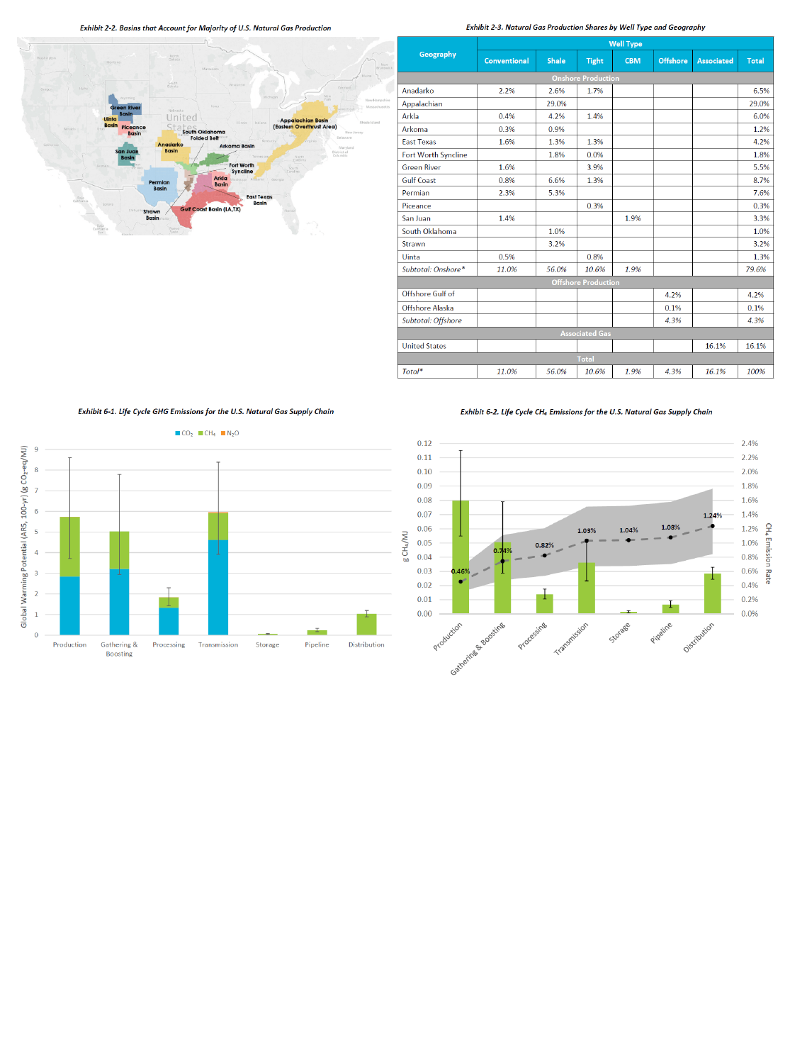
BLM 2021
(a) (b)
(c) (d)
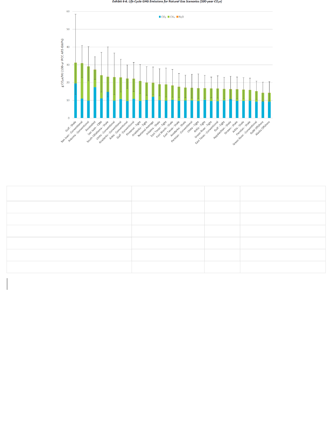
BLM 2021
(e)
Figure 4-1. NETL Report Exhibits for LCA Estimates
Table 4-6. GHG Emissions Factors for Federal Gas Production
g = grams, kg = kilograms, MJ = megajoule, gal = gallons.
Direct methane emissions factor is included in the direct CO e factor as CO e.
Report year emissions and projected emissions from BLM gas leasing authorizations and permitting actions
are based on ONRR records of actual gas production. Table 4-7 shows a summary of the ONRR production
data from states that reported federal gas production during the past 5 years. The table also shows total
U.S. gas production (federal and nonfederal) to illustrate the percentage of federal gas relative to the U.S.
total (% U.S. Total) and the percentage of federal gas that comes from the various federal gas producing
states (% Federal). The U.S. total data includes all gas produced from both onshore and offshore sources.
The percent total calculations are based on the 5-year average data column (see example calculation in table
notes).
Category Units CO e Reference
2
Direct (extraction) g CO e/MJ
2
5.732 Cooney et al. 2019
Direct (methane) g CH /MJ (0.08)
4
2.88 Cooney et al. 2019
Indirect (gather & boost) g CO e/MJ
2
5.036 Cooney et al. 2019
Indirect (processing) g CO e/MJ
2
1.854 Cooney et al. 2019
Indirect (transport & storage) g CO e/MJ
2
7.278 Cooney et al. 2019
End Use (combustion) kg CO e/scf
2
0.0545 40 CFR Part 98
2 2

BLM 2021
Table 4-7. Federal Gas Production (Mcf)
Ex: % U.S. Total for CO (1.95%) = (638,030,405 / 32,666,894,200 * 100) & % Federal CO (19.28%) = (638,030,405 /
3,308,841,094 * 100)
28,400,049,000 29,237,825,000 33,008,867,000 36,515,188,000 36,172,542,000 32,666,894,200 100% NA
3,300,221,597 3,236,718,007 3,327,281,643 3,386,536,791 3,293,447,433 3,308,841,094 10.13% 100%
1,459,623,235 1,406,667,426 1,419,371,754 1,291,223,275 1,210,670,154 1,357,511,169 4.16% 41.03%
782,795,288 786,532,574 885,024,132 1,047,716,286 1,141,952,863 928,804,229 2.84% 28.07%
637,490,392 650,811,134 647,023,114 663,121,139 591,706,248 638,030,405 1.95% 19.28%
235,202,222 197,763,804 175,152,176 157,320,280 139,276,421 180,942,981 0.55% 5.47%
45,796,092 55,516,094 68,403,067 88,297,683 84,420,597 68,486,707 0.21% 2.07%
33,291,605 31,245,879 27,612,984 27,677,111 21,409,926 28,247,501 0.09% 0.85%
13,270,317 18,172,556 21,156,381 29,535,558 27,499,806 21,926,924 0.07% 0.66%
14,565,324 16,345,944 14,977,468 17,782,538 17,993,335 16,332,922 0.05% 0.49%
18,466,624 15,772,758 15,125,112 14,920,403 14,478,710 15,752,721 0.05% 0.48%
12,846,836 12,337,060 11,695,098 11,116,341 10,442,392 11,687,545 0.04% 0.35%
13,662,395 11,781,386 10,215,707 10,471,581 9,265,633 11,079,340 0.03% 0.33%
12,424,517 11,001,930 10,121,088 8,943,097 8,215,842 10,141,295 0.03% 0.31%
11,877,207 10,960,592 11,042,091 9,810,633 6,785,129 10,095,130 0.03% 0.31%
4,223,135 3,915,997 3,761,159 3,555,465 3,224,742 3,736,100 0.01% 0.11%
347,161 3,925,058 3,602,566 2,245,117 3,649,083 2,753,797 0.01% 0.08%
1,368,307 1,286,369 1,198,808 1,237,833 1,104,798 1,239,223 0% 0.04%
1,689,070 1,233,049 948,608 877,074 772,480 1,104,056 0% 0.03%
403,612 380,157 273,389 267,817 224,962 309,987 0% 0.01%
382,866 614,946 83,249 25,152 11,465 223,536 0% 0.01%
156,876 148,092 138,262 123,196 116,552 136,596 0% 0%
156,228 122,040 112,145 106,260 97,191 118,773 0% 0%
137,852 138,197 119,371 82,685 56,494 106,920 0% 0%
26,713 28,755 110,760 68,498 54,450 57,835 0% 0%
6,042 7,647 7,797 7,559 5,722 6,953 0% 0%
9,233 6,532 3,638 2,584 2,196 4,837 0% 0%
1,813 1,772 1,708 1,617 10,240 3,430 0% 0%
635 259 11 9 2 183 0% 0%
2016 2017 2018 2019 2020
5-Year
Average
%
U.S.
Total
%
Federal
U.S.
Total
Federal
Total
WY
NM
CO
UT
ND
TX
LA
AK
OK
MT
AL
AR
CA
KS
OH
MI
SD
MS
ID
VA
KY
WV
PA
NY
IL
NV
NE
Area

BLM 2021
4.6 Short-Term Oil and Gas Projections
The short-term projections for oil and gas emissions are based on analyses of three authorization scopes
that exist for potential oil and gas production. These include (1) leased federal lands that are
, (2) approved , and (3) leased lands from competitive lease
sales expected to occur over the next annual reporting cycle (12 months). As was the case for coal, here too
the BLM is assuming that all oil and gas developed is consumed in the same year. When initiating a planning
action in an area of potential oil and gas development, the BLM may produce an analysis of the fluid mineral
potential known as a (RFD) for oil and gas development for
the specific geographic area. An RFD is typically constructed to support the management actions developed
for a field or district office’s resource management plan. The RFD provides an estimate of development
potential and growth rates within the specified region based on several indicators, including the estimated
hydrocarbon potential, operator surveys, existing development trends, various economics forecasts, and
basin or geology factors, among others. These documents typically provide 20+ years of oil and gas
development estimates and have traditionally been used to inform decisions on areas open and closed for
leasing and the need for implementing stipulations, conditions of approval, or mitigation measures. The
RFDs that are currently available, although useful for informing management actions and tracking limits of
analysis for a particular region, are not useful for estimating GHG emissions across all BLM-managed
mineral estate in a particular year because of their differing years of analysis, projection methodologies, and
management objectives. The BLM does not currently have an up-to-date RFD that covers the entire federal
onshore mineral estate. Due to the inconsistencies among available RFDs and a lack of an RFD for all federal
mineral producing regions, the individual RFDs or a summation of all available RFDs may not be used to
derive a single replicable methodology from which to make projections, which is one of the goals of this
report. Thus, for the purposes of this report, a more representative and consistent approach for making
projections that captures the implications of different levels of development and production across the
entirety of the federal mineral estate was employed.
Each of the authorization scopes previously described relies in part on the most recent 5-year average
dataset of federal mineral statistics developed by the BLM in combination with the previously identified
external sources of fossil fuel production data. The development statistics include both internal BLM
tracking data, such as annual lease acres and held-by-production rates, APD approval counts, rates, and
counts, as well as an analysis of external well completion and production rates for individual
wells in states reporting federal oil and gas production. Additional parameters are calculated from the
internal statistics to aid in the projection calculations and to provide custom metrics for tracking purposes as
shown in Table 4-8.
Table 4-8. 5-Year Federal Oil and Gas Statistics (BLM Totals)
held-by-
production applications for permit to drill (APDs)
Reasonably Foreseeable Development Scenario
[19 ]
spud
producible well
27,207,018 25,742,991 25,552,475 26,287,326 26,604,169 26,278,796
12,771,830 12,790,557 12,794,552 12,915,006 12,711,111 12,796,611
46.94% 49.69% 50.07% 49.13% 47.78% 48.7%
577,317 1,114,218 1,253,369 2,245,906 1,871,962 1,412,553
2,184 2,486 3,388 3,181 4,226 3,928
847 1,428 1,919 1,995 1,486 1,533
2016 2017 2018 2019 2020
5-Year
Average
Acres Under Lease
Producing Acres
Acres Held by Production (%) *
New Lease Acres (sold)
Number of APDs Approved
Number of Wells Spud
Statistic
BLM 2021
Source: BLM Oil and Gas Statistics.
"*" Denotes calculated parameter.
The BLM analyzed 10 years (2011-2020) of external data from the IHS Markit Enerdeq database (commercial
source) for oil and gas wells in federal mineral producing states. The analysis of the individual wells
provided an estimate of the total potential mineral yield, or , and the
associated rates that could be expected from any new wells developed within the authorization
scopes analyzed in this report. Producing the EUR and decline estimates was necessary because life-of-
project production is a reasonably foreseeable outcome from existing and future authorizations if economic
quantities of federal minerals exist within any authorization scope.
Enerdeq provides subscription-based access to more than 5 million completions and 2.5 million production
entities and provides an adequate sample size for most regions to apply statistical methods for determining
the EUR. Initially, the BLM made queries to obtain the American Petroleum Institute (API) well identifiers for
all new wells completed within the last 10 years. The 10-year timeframe was chosen to capture the changes
in characteristics for wells developed before and after the advent and widespread adoption of horizontal
drilling and hydraulic fracturing completion techniques. The queried data was scrubbed to eliminate
nontarget wells (e.g., injection, water) and then organized by state to query 10 years of production data. This
query provided the individual well production-by-age data that was necessary to develop the decline curve
profiles and provide for cumulative production estimates over the life of a well. Oil and gas wells typically
produce high quantities of minerals initially, followed by a period of rapid decline that settles into a very
shallow decline over the remainder of their economic life. The BLM applied regression analysis techniques to
the production data to generate a typical decline equation for wells in each state. The EUR for each state
was calculated for an estimated life span of 30 years. These EUR volumes were then applied to the
estimated number of new wells projected for the applicable authorization boundaries in each state to
estimate cumulative or life-of-project GHG emissions. The decline curve formulas are also useful for
estimating existing held-by-production projections as described later. Table 4-9 presents some of the IHS
data highlights that went into the BLM's analysis, and Figure 4-2 shows the results of the decline analysis for
the selected state.
94,096 94,434 96,199 96,356 96,110 95,437
0.245 0.312 0.3215 0.3119 0.3131 0.3007
189,524 181,534 185,671 186,699 192,262 187,136
95,441 87,112 89,485 90,356 96,165 91,711
4,473.3 1,764 608.9 1,172.7 1,090 1,823
252.21 251.71 277.3 309.45 313.64 280.86
418.92 421.03 404.8 439.91 407.76 418.5
1,479 1,611 3,102 6,294 2,897 3,133
estimated ultimate recovery (EUR)
decline
2016 2017 2018 2019 2020
5-Year
Average
Number of Producible Wells
Federal Wells per Acre *
Total Potential Wells *
Potential New Wells *
Potential Development Years *
Total CO2e Emissions (Mt) *
CO2e Emissions (tonnes/prod
acre) *
Potential New Lease Wells *
Statistic

BLM 2021
Table 4-9. IHS Markit Enerdeq Data as Analyzed by BLM
Data is representative of all wells (federal and nonfederal) drilled and producing within the analyzed period.
Active status assigned to states with development rates of approximately 1,000 or more wells per year.
1,429 226 1,203 2.11% 588 2.85% 655 2
775 753 23 0.15% 175 0.06% 503 4
4,628 1,725 2,903 0.05% 270 2.48% 3,167 2
16,815 Active 14,807 2,008 0.19% 1,315 0.03% 1,062 5
18,560 Active 9,487 9,073 5.16% 17,055 4.75% 17,798 15
11 11 0 0.00% 0 0.00% 0 1
15,786 Active 15,395 391 0.53% 3,916 0.15% 1,215 12
10,304 Active 6,873 3,431 3.05% 3,711 11.16% 4,557 1
368 217 151 0.09% 188 0.02% 97 2
1,319 1,220 99 0.38% 690 0.05% 316 3
1,241 421 820 0.45% 788 0.05% 757 14
16,035 Active 123 15,912 16.01% 13,890 2.73% 13,855 1
479 477 2 0.04% 254 0.00% 1 6
11,482 Active 4,610 6,872 7.08% 9,811 2.70% 10,043 6
6 6 0 0.00% 0 0.00% 0 1
986 973 13 0.00% 838 0.00% 790 1
4,091 1,337 2,754 0.72% 2,807 6.13% 3,697 2
20,081 Active 7,158 12,923 5.07% 13,408 6.97% 14,245 14
4 4 0 0.00% 0 0.00% 0 1
13,971 Active 4,629 9,342 0.21% 5,396 21.80% 12,959 2
65 5 60 0.02% 44 0.00% 31 4
107,473 Active 49,715 57,758 55.24% 46,383 28.48% 47,330 15
6,217 5,851 366 0.99% 4,672 0.81% 4,672 10
3,877 845 3,032 0.42% 2,720 5.75% 3,663 1
9,975 Active 7,564 2,411 2.04% 7,038 3.02% 7,234 13
265,978 134,432 131,547 100% 135,957 100% 148,647 138
New Well
Count
Dev
Status
Vertical Horizontal
Percent
Oil
Prod
Oil Prod
Record
Cnt
Percent
Gas
Prod
Gas
Prod
Record
Cnt
No. of
Basin /
Formations
AK
AL
AR
CA
CO
ID
KS
LA
MI
MS
MT
ND
NE
NM
NV
NY
OH
OK
OR
PA
SD
TX
UT
WV
WY
Totals
State
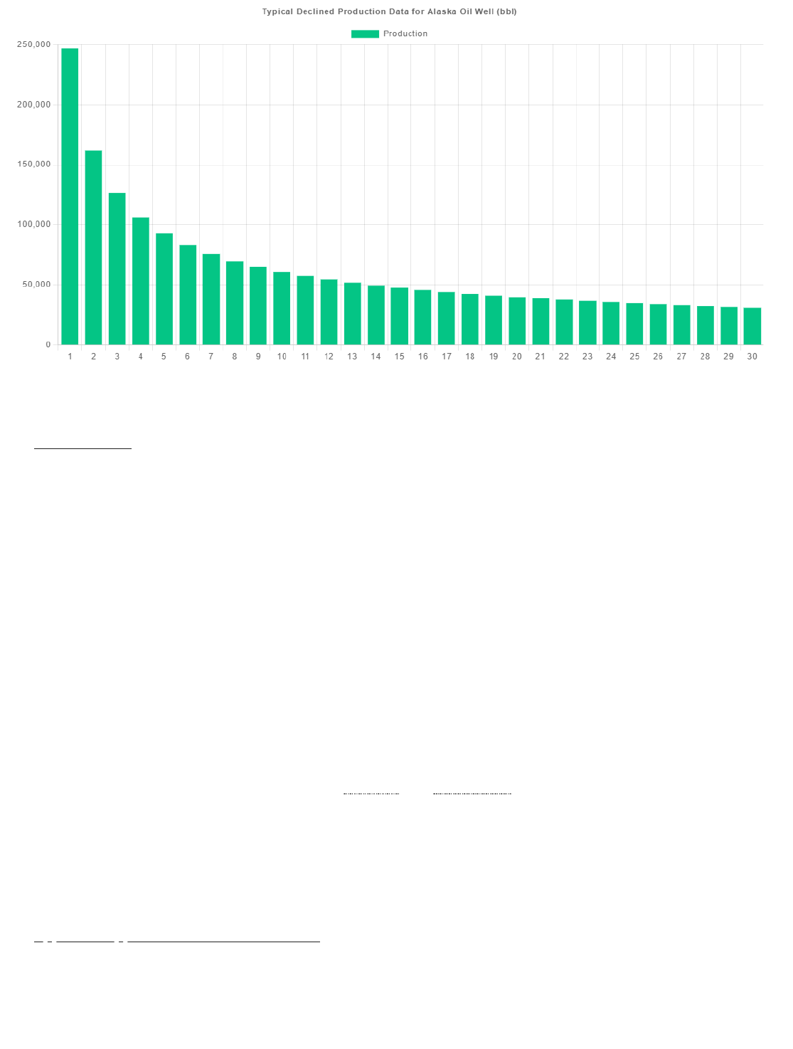
BLM 2021
W e l l D e c l i n e P r o d u c t i o n Y e a r S e r i e s S u m = 1 , 9 1 0 , 5 9 8 . 0 2 3
Figure 4-2. State Oil and Gas Decline Curves (Alaska - Oil)
Leased Lands
To estimate the potential GHG emissions resulting from leased lands held-by-production, the BLM applies the
derived decline curves on a relative basis to the report year production levels and projects out for an
additional 30 years (the assumed life-of-project period) for each applicable state. The decline curves for any
state are statistically valid for an average “new” well; however, the held-by-production data is representative
of wells at various ages. Thus applying the decline curve to existing field-wide production would most likely
underrepresent future cumulative emissions. The decline data show that newer wells are far more
productive in their first few years of life than over the entire life of the project period, and thus it is generally
assumed that for any region with active development, the newer wells are driving production. For these
areas, the BLM assumed a field-wide decline age of 5 years. For a majority of the decline data, the 5-year
mark lands squarely at the heel of the harmonic shaped curves (see Figure 4-2, year 5) and should
correspond with a moderate gradual decline that could be expected at field-wide scales with active
development. For all other regions, the decline age was assumed to be 10 years (very shallow decline,
leading to sustained production over the projection period). Additionally, this analysis conservatively
assumes that all existing wells on leases held-by-production will continue to produce for another 30 years,
even though it is highly likely that some will be and . This fact can be clearly seen in the
data contained in Table 4-8; even though the BLM recorded 1,533 well spuds per year on average over the 5-
year period, the producible well counts only increased by 2,014 wells over the entire 5-year period. Its likely
that some of the recorded spuds came up dry leading to a smaller increment in the producible well counts,
just as it is likely that some of the producible wells on record reached the end of their economic lives (i.e., no
longer considered producible), and were thus subtracted from this count.
Approved Applications for Permit to Drill
To estimate the potential GHG emissions resulting from approved APDs, the BLM uses the last 2 years of
approved APD counts minus the spuds recorded for the same period. Here the BLM is breaking from the
general approach in this report of using 5-year average data for making projections in acknowledgement that
plugged abandoned

BLM 2021
APDs are only valid for 2 years (absent extensions that can be granted for an additional 2 years with
appropriate justification). In general, the BLM statistics show that spud counts lag APD approvals across the
states, and therefore it is reasonable to assume that the delta between the two metrics is enough to cover
any potential extensions and subsequent development that may arise during the reporting period (i.e., the
next 12 months). The remaining APD counts are multiplied by the corresponding decline curve equation that
was derived for each state.
Potential Future Leasing
Estimates of potential GHG emissions resulting from any future leasing are relatively speculative. In terms of
emissions, the BLM is assuming that full development of the leased would occur concurrently within
the same sale (report) year. While this assumption does not reflect a typical timeline for oil and gas
development, it is simplifying for projection purposes and allows the BLM to evaluate the potential emissions
for any authorizations made. Here, the BLM relies on the 5-year average of the acres held by production, the
annual total leased acres, and the calculated well density (wells per acre) on the federal mineral estate.
Additionally, for some states with leased lands where the 5-year average statistics fall below a threshold
minimum, the BLM assumes a minimum leased acreage to conservatively estimate potential emissions. The
minimum thresholds are 100 acres leased for states with less than 4,000 acres currently leased, and 2,560
acres leased for states with more than 4,000 acres currently leased for which the 5-year leasing average is
less than the minimum itself. The statistical annual lease acres data (5-year average) or the alternative
minimum lease acres is used to estimate the number of wells for potentially leased lands which are then
multiplied by the corresponding decline curve data for each state to obtain the estimated life-of-project
production and emissions.
4.7 Long-Term Federal Fossil Fuel Mineral Emissions Projections
The emission estimates from the federal mineral estate authorization boundaries previously outlined present
current emissions and projected emissions based on potential development and production volumes over the
short term. As discussed at the beginning of this section, the BLM is using data from EIA's AEO report to
estimate potential long-term emissions (to year 2050). The AEO is developed using the National Energy
Modeling System (NEMS), an integrated model that captures interactions of economic changes and energy
supply, demand, and prices. The AEO is published to satisfy the Department of Energy Organization Act of
1977, which requires EIA’s Administrator to prepare annual reports on trends and projections for energy use
and supply. The AEO explores several scenarios that capture alternative policy-based cases that can be
compared to the reference case, which represents EIA’s best assessment of how U.S. and world energy
markets will operate through 2050. The reference case examines a future characterized by slower growth in
energy consumption (due to energy efficiency increases) and by increasing energy supply due to
technological progress in the renewable, oil, and natural gas energy sectors. The reference case is also the
baseline scenario from which all other side-case estimates are made. The most current version of the report
(AEO 2021) was used to supplement this report. Note: Projections in the AEO are not predictions of what will
happen, but rather, they are modeled projections of what may happen given certain assumptions. The major
underlying assumption for the application of any AEO scenario data is that the ratio of federal and nonfederal
mineral production is fixed at the current 5-year average for each state going forward. The five-year average
was chosen to alleviate any annual variability in production that can arise for any number of reasons. For
each year of AEO data, which is inclusive of total (federal and nonfederal) production, the BLM is applying the
5-year average federal fraction for each mineral type to forecast long-term federal mineral production from
which to estimate emissions. Overall, this forecast method is useful for analyzing long-term trends in GHG
emissions and comparing the levels to specific climate change policy milestones to ascertain reasonable
progress.
parcels

BLM 2021
4.8 Uncertainties in Emissions Estimates
This report relies on life-cycle emissions estimates produced in part by the DOE NETL (as previously cited).
The life-cycle estimates produced by the BLM cover broad activities used to represent recovery and
processing of federal minerals, including lease exploration, construction, well drilling and completion,
production, processing, transportation, and end use. The BLM acknowledges that operational diversity,
product variations, and broad geographic distribution of the federal mineral estate introduces some
uncertainty into the simplifying assumptions and approximation methodologies used to estimate emissions
in this report. This acknowledgement is not intended to dispute the validity of the estimates but to help
prioritize efforts to improve the accuracy of future iterations of this report. For some of the current
estimates, such as CO emissions from energy-related combustion activities, the impact of uncertainties on
overall emission estimates is believed to be relatively small. For some other limited categories of emissions,
including the assumptions used to estimate production and project future emissions, the following
uncertainties could have a larger impact on the estimates.
The uncertainties inherent to the sourced LCA data, which is unavoidably propagated in the BLM
estimates.
Uncertainty in global warming potential (GWP) factors, which may be up to + or - 40% and may change
often due to updated scientific understanding.
Unknowable factors about actual or future development localities, methodologies, and production rates.
The exact nature of energy sources and amounts used in production, transportation, and processing
systems.
How the produced federal minerals are ultimately transformed and used.
The overall energy density of the produced federal mineral estate (used in emissions calculations).
The exact nature of any control technology that may be utilized at direct or indirect activity locations.
Regulatory and policy posture changes with respect to GHGs by governments or agencies with authority
for such matters.
The BLM is making a broad but concerted effort to utilize and present the best data available for the
emissions estimates in this report. As new information becomes available, the BLM will continue to improve
and revise its emission estimates, methodologies, and assumptions as appropriate. Ultimately, these
estimates are subject to many influences that are largely beyond the BLM’s practical control. Unforeseen
changes in several factors such as geologic conditions, drilling technology, global and national economics,
energy demand, and laws and policies enacted at the federal, state, and local level could result in different
outcomes than those projected in this assessment.
* * *
2

BLM 2021
This chapter provides direct and indirect GHG emission estimates for both existing and projected federal
fossil fuel production. Existing emissions estimates show the GHGs emitted from the assumed consumption
of each fossil fuel based on production statistics from the previous fiscal year for all producing wells and
mines. The projected emissions include both, short- and long-term estimates based on the methodologies
discussed in the previous chapter.
5.1 Short-Term Coal Emissions
Table 5-1 presents the emissions from coal production on the federal mineral estate in FY 2020, which result
from multiplying the representative emission factors from Table 4-1 by the state-specific production amounts
from Table 4-2. The estimates presented here include emissions from the typical coal lifecycle, including
emissions arising from activities outside of the BLM's jurisdiction (such as emissions associated with coal
exports). Table 5-2 shows the short-term emissions projections from reasonably foreseeable coal
production in the 8 states where the BLM has currently authorized coal leasing.
Table 5-1. Federal Coal Emissions - 2020 (Mt)
Production units = tons.
LCA CH is included in the Extraction CO e estimates as CO e.
U.S. Total is both federal and nonfederal data, shown for illustration purposes.
534,302,000 0.8442 33.116 NA 28.7187 1,186.24 1,248.07
246,391,712 0.0588 4.846 NA 27.3627 458.74 490.94
206,576,818 0.0303 3.0739 NA 24.4009 366.31 393.78
13,407,510 0.002 0.1995 NA 1.5837 23.77 25.55
12,241,079 0.0119 0.3192 NA 0.5136 30.63 31.46
8,987,084 0.0142 0.557 NA 0.4831 27.88 28.92
2,996,726 0.0004 0.0446 NA 0.354 5.31 5.71
1,963,242 0 0.5863 NA 0.0247 4.36 4.97
145,052 0 0.0433 NA 0.0018 0.32 0.37
74,201 0 0.0222 NA 0.0009 0.16 0.18
4 2 2
2020
Production
LCA
CH4
Extraction
CO2e
Processing
CO2e
Transport
CO2e
Combustion
CO2e
Total
CO2e
U.S. Total
Federal Total
WY
MT
UT
CO
ND
NM
AL
OK
Area
5.0 GHG Emissions and Projections from BLM-Authorized Actions

BLM 2021
Table 5-2. Federal Coal Emissions - Projected Short-Term
Life-of-Project (Mt)
EUR means Estimated Ultimate Recovery (production), units are short tons.
LCA CH is included in the Extraction CO e estimates as CO2 e.
Emissions are projected for a single future year due to a lack of verifiable remaining coal reserve data.
5.2 Short-Term Oil and Gas Emissions
Tables 5-3 and 5-6 present the short-term LCA emissions from oil and gas production on the federal mineral
estate in FY 2020 (held-by-production), which result from multiplying the representative emission factors
from Tables 4-4 and 4-6 by the state-specific production amounts from Tables 4-5 and 4-7, respectively. The
estimates presented here include emissions from the full oil and gas lifecycle, including emissions arising
from activities outside of the BLM's jurisdiction (such as emissions associated with refining and
processing). Tables 5-4, 5-5, 5-7, and 5-8 show the short-term LCA emissions projections from reasonably
foreseeable oil and gas production on the held-by-production lands for the next twelve months and over the
estimated life-of-project.
274,368,909 0.2955 5.6593 0 30.4683 509.92 546.06
229,340,768 0.0336 3.4126 NA 27.0897 406.6739 437.18
15,737,608 0.2342 0.2342 NA 1.8589 27.9064 30
12,602,926 0.0122 0.3287 NA 0.5288 31.5384 32.4
9,522,631 0.015 0.5902 NA 0.5118 29.5385 30.64
3,686,029 0.0005 0.0548 NA 0.4354 6.5362 7.03
3,088,896 0 0.9224 NA 0.0388 6.8579 7.82
272,075 0 0.0812 NA 0.0034 0.6041 0.69
117,976 0 0.0352 NA 0.0015 0.2619 0.3
4 2 2
EUR
Production
LCA
CH4
Extraction
CO2e
Processing
CO2e
Transport
CO2e
Combustion
CO2e
Total
CO2e
Federal Total
WY
MT
UT
CO
ND
NM
AL
OK
Area

BLM 2021
Table 5-3. Federal Oil Emissions - Held-By-Production Lands
2020 (Mt)
Production units (bbl).
U.S. Total is both federal and nonfederal data, shown for illustration purposes.
4,140,738,000 5.52 329.1736 196.1618 42.0085 1,795.82 2,363.16
314,421,357 0.3489 24.9954 14.8953 3.1899 136.36 179.44
197,468,433 0.2191 15.698 9.3548 2.0034 85.64 112.7
49,245,858 0.0546 3.9149 2.333 0.4996 21.36 28.11
39,263,016 0.0436 3.1213 1.86 0.3983 17.03 22.41
9,507,307 0.0105 0.7558 0.4504 0.0965 4.12 5.42
6,572,944 0.0073 0.5225 0.3114 0.0667 2.85 3.75
6,412,327 0.0071 0.5098 0.3038 0.0651 2.78 3.66
2,900,906 0.0032 0.2306 0.1374 0.0294 1.26 1.66
952,457 0.0011 0.0757 0.0451 0.0097 0.41 0.54
627,964 0.0007 0.0499 0.0297 0.0064 0.27 0.36
449,725 0.0005 0.0358 0.0213 0.0046 0.2 0.26
283,556 0.0003 0.0225 0.0134 0.0029 0.12 0.16
237,328 0.0003 0.0189 0.0112 0.0024 0.1 0.13
231,409 0.0003 0.0184 0.011 0.0023 0.1 0.13
101,983 0.0001 0.0081 0.0048 0.001 0.04 0.05
98,387 0.0001 0.0078 0.0047 0.001 0.04 0.05
18,477 0 0.0015 0.0009 0.0002 0.01 0.01
17,410 0 0.0014 0.0008 0.0002 0.01 0.01
10,333 0 0.0008 0.0005 0.0001 0 0
8,953 0 0.0007 0.0004 0.0001 0 0
8,579 0 0.0007 0.0004 0.0001 0 0
3,269 0 0.0003 0.0002 0 0 0
569 0 0 0 0 0 0
164 0 0 0 0 0 0
3 0 0 0 0 0 0
2020
Production
LCA
CH4
Extraction
CO2e
Processing
CO2e
Transport
CO2e
Combustion
CO2e
Total
CO2e
U.S. Total
Federal Total
NM
WY
ND
CA
CO
UT
MT
AK
OK
LA
TX
NV
MS
KS
SD
NE
AL
MI
OH
IL
KY
PA
ID
AR
Area

BLM 2021
Table 5-4. Federal Oil Emissions - Held-By-Production Lands
Projected 12-Months (Mt)
Production units (bbl).
238,642,669 0.2647 18.9714 11.3055 2.4213 103.48 136.18
145,466,545 0.1614 11.5641 6.8913 1.4758 63.09 83.02
32,188,451 0.0357 2.5589 1.5249 0.3266 13.96 18.37
37,946,927 0.0421 3.0166 1.7977 0.385 16.46 21.66
7,758,321 0.0086 0.6168 0.3675 0.0787 3.36 4.42
5,122,593 0.0057 0.4072 0.2427 0.052 2.22 2.92
2,668,212 0.003 0.2121 0.1264 0.0271 1.16 1.53
4,662,063 0.0052 0.3706 0.2209 0.0473 2.02 2.66
898,844 0.001 0.0715 0.0426 0.0091 0.39 0.51
568,214 0.0006 0.0452 0.0269 0.0058 0.25 0.33
423,350 0.0005 0.0337 0.0201 0.0043 0.18 0.24
262,376 0.0003 0.0209 0.0124 0.0027 0.11 0.15
215,097 0.0002 0.0171 0.0102 0.0022 0.09 0.12
213,400 0.0002 0.017 0.0101 0.0022 0.09 0.12
92,748 0.0001 0.0074 0.0044 0.0009 0.04 0.05
93,303 0.0001 0.0074 0.0044 0.0009 0.04 0.05
17,134 0 0.0014 0.0008 0.0002 0.01 0.01
16,247 0 0.0013 0.0008 0.0002 0.01 0.01
9,650 0 0.0008 0.0005 0.0001 0 0
8,012 0 0.0006 0.0004 0.0001 0 0
7,626 0 0.0006 0.0004 0.0001 0 0
2,898 0 0.0002 0.0001 0 0 0
504 0 0 0 0 0 0
151 0 0 0 0 0 0
3 0 0 0 0 0 0
Projected Production
(12 months)
LCA
CH4
Extraction
CO2e
Processing
CO2e
Transport
CO2e
Combustion
CO2e
Total
CO2e
Federal Total
NM
ND
WY
CA
UT
MT
CO
AK
OK
LA
TX
MS
NV
SD
KS
NE
AL
MI
IL
OH
KY
PA
ID
AR
Area

BLM 2021
Table 5-5. Federal Oil Emissions - Held-By-Production Lands
Projected Life-of-Project (Mt)
EUR Production units (bbl).
1,860,945,007 2.0648 147.94 88.16 18.88 807.09 1,062.08
978,834,961 1.086 77.8138 46.371 9.9305 424.52 558.64
333,952,435 0.3705 26.548 15.8205 3.388 144.83 190.59
302,793,218 0.336 24.071 14.3444 3.0719 131.32 172.81
78,842,196 0.0875 6.2677 3.735 0.7999 34.19 44.99
47,435,886 0.0526 3.771 2.2472 0.4812 20.57 27.07
42,837,144 0.0475 3.4054 2.0294 0.4346 18.58 24.45
27,521,847 0.0305 2.1879 1.3038 0.2792 11.94 15.71
17,275,101 0.0192 1.3733 0.8184 0.1753 7.49 9.86
8,180,577 0.0091 0.6503 0.3875 0.083 3.55 4.67
7,991,271 0.0089 0.6353 0.3786 0.0811 3.47 4.57
4,388,383 0.0049 0.3489 0.2079 0.0445 1.9 2.5
3,712,495 0.0041 0.2951 0.1759 0.0377 1.61 2.12
2,949,851 0.0033 0.2345 0.1397 0.0299 1.28 1.68
1,768,578 0.002 0.1406 0.0838 0.0179 0.77 1.01
1,444,897 0.0016 0.1149 0.0685 0.0147 0.63 0.83
290,965 0.0003 0.0231 0.0138 0.003 0.13 0.17
288,360 0.0003 0.0229 0.0137 0.0029 0.13 0.17
172,119 0.0002 0.0137 0.0082 0.0017 0.07 0.09
142,902 0.0002 0.0114 0.0068 0.0014 0.06 0.08
76,320 0.0001 0.0061 0.0036 0.0008 0.03 0.04
36,651 0 0.0029 0.0017 0.0004 0.02 0.03
6,379 0 0.0005 0.0003 0.0001 0 0
2,422 0 0.0002 0.0001 0 0 0
49 0 0 0 0 0 0
EUR
Production
LCA
CH4
Extraction
CO2e
Processing
CO2e
Transport
CO2e
Combustion
CO2e
Total
CO2e
Federal Total
NM
ND
WY
CA
UT
MT
CO
AK
OK
LA
TX
MS
NV
SD
KS
NE
AL
MI
IL
OH
KY
PA
ID
AR
Area

BLM 2021
Table 5-6. Federal Gas Emissions - Held-By-Production Lands
2020 (Mt)
Production units (Mcf).
U.S. Total is both federal and nonfederal data, shown for illustration purposes.
36,172,542,000 3.1325 224.444 72.5958 482.1709 1,947.21 2,726.42
3,293,447,433 0.2852 20.4352 6.6097 43.9008 177.29 248.24
1,210,670,154 0.1048 7.512 2.4297 16.1379 65.17 91.25
1,141,952,863 0.0989 7.0856 2.2918 15.2219 61.47 86.07
591,706,248 0.0512 3.6714 1.1875 7.8873 31.85 44.6
139,276,421 0.0121 0.8642 0.2795 1.8565 7.5 10.5
84,420,597 0.0073 0.5238 0.1694 1.1253 4.54 6.36
27,499,806 0.0024 0.1706 0.0552 0.3666 1.48 2.07
21,409,926 0.0019 0.1328 0.043 0.2854 1.15 1.61
17,993,335 0.0016 0.1116 0.0361 0.2398 0.97 1.36
14,478,710 0.0013 0.0898 0.0291 0.193 0.78 1.09
10,442,392 0.0009 0.0648 0.021 0.1392 0.56 0.79
9,265,633 0.0008 0.0575 0.0186 0.1235 0.5 0.7
8,215,842 0.0007 0.051 0.0165 0.1095 0.44 0.62
6,785,129 0.0006 0.0421 0.0136 0.0904 0.37 0.52
3,649,083 0.0003 0.0226 0.0073 0.0486 0.2 0.28
3,224,742 0.0003 0.02 0.0065 0.043 0.17 0.24
1,104,798 0.0001 0.0069 0.0022 0.0147 0.06 0.08
772,480 0.0001 0.0048 0.0016 0.0103 0.04 0.06
224,962 0 0.0014 0.0005 0.003 0.01 0.01
116,552 0 0.0007 0.0002 0.0016 0.01 0.01
97,191 0 0.0006 0.0002 0.0013 0.01 0.01
56,494 0 0.0004 0.0001 0.0008 0 0
54,450 0 0.0003 0.0001 0.0007 0 0
11,465 0 0.0001 0 0.0002 0 0
10,240 0 0.0001 0 0.0001 0 0
5,722 0 0 0 0.0001 0 0
2,196 0 0 0 0 0 0
2 0 0 0 0 0 0
2020
Production
LCA
CH4
Extraction
CO2e
Processing
CO2e
Transport
CO2e
Combustion
CO2e
Total
CO2e
U.S. Total
Federal Total
WY
NM
CO
UT
ND
LA
TX
AK
OK
MT
AL
AR
CA
OH
KS
MI
SD
MS
VA
KY
WV
PA
ID
NV
NY
IL
NE
Area

BLM 2021
Table 5-7. Federal Gas Emissions - Held-By-Production Lands
Projected 12-Months (Mt)
Production units (Mcf).
2,664,011,775 0.2306 16.5296 5.3463 35.5107 143.4 200.79
1,029,379,035 0.0891 6.3871 2.0659 13.7214 55.41 77.58
908,057,421 0.0786 5.6343 1.8224 12.1042 48.88 68.44
423,053,787 0.0366 2.625 0.849 5.6392 22.77 31.88
120,684,134 0.0105 0.7488 0.2422 1.6087 6.5 9.1
68,883,035 0.006 0.4274 0.1382 0.9182 3.71 5.19
24,647,247 0.0021 0.1529 0.0495 0.3285 1.33 1.86
19,594,579 0.0017 0.1216 0.0393 0.2612 1.05 1.47
16,540,344 0.0014 0.1026 0.0332 0.2205 0.89 1.25
13,207,446 0.0011 0.0819 0.0265 0.1761 0.71 0.99
9,690,823 0.0008 0.0601 0.0194 0.1292 0.52 0.73
8,566,139 0.0007 0.0532 0.0172 0.1142 0.46 0.64
7,593,998 0.0007 0.0471 0.0152 0.1012 0.41 0.57
5,704,256 0.0005 0.0354 0.0114 0.076 0.31 0.43
2,931,628 0.0003 0.0182 0.0059 0.0391 0.16 0.22
3,134,597 0.0003 0.0194 0.0063 0.0418 0.17 0.24
1,076,544 0.0001 0.0067 0.0022 0.0144 0.06 0.08
729,876 0.0001 0.0045 0.0015 0.0097 0.04 0.06
211,481 0 0.0013 0.0004 0.0028 0.01 0.01
107,753 0 0.0007 0.0002 0.0014 0.01 0.01
89,854 0 0.0006 0.0002 0.0012 0 0
49,231 0 0.0003 0.0001 0.0007 0 0
50,781 0 0.0003 0.0001 0.0007 0 0
10,640 0 0.0001 0 0.0001 0 0
5,652 0 0 0 0.0001 0 0
9,352 0 0.0001 0 0.0001 0 0
2,140 0 0 0 0 0 0
2 0 0 0 0 0 0
Projected Production
(12 months)
LCA
CH4
Extraction
CO2e
Processing
CO2e
Transport
CO2e
Combustion
CO2e
Total
CO2e
Federal Total
WY
NM
CO
UT
ND
LA
TX
AK
OK
MT
AL
AR
CA
KS
OH
MI
SD
MS
VA
KY
PA
WV
ID
NY
NV
IL
NE
Area

BLM 2021
Table 5-8. Federal Gas Emissions - Held-By-Production Lands
Projected Life-of-Project (Mt)
EUR Production units (Mcf).
Tables 5-9 through and 5-12 present the short-term projections of LCA emissions for reasonably foreseeable
oil and gas production from approved APDs. The estimates shown assume all APDs will be drilled,
completed, and have completed a full 12 months of production during the next 12 months.
27,524,613,884 2.3835 170.79 55.24 366.9 1,481.69 2,074.62
12,657,678,353 1.0961 78.5386 25.4031 168.7237 681.38 954.05
8,244,637,251 0.714 51.1565 16.5464 109.8989 443.82 621.42
2,565,021,869 0.2221 15.9155 5.1478 34.1911 138.08 193.33
1,628,264,872 0.141 10.1031 3.2678 21.7044 87.65 122.73
699,674,711 0.0606 4.3414 1.4042 9.3265 37.66 52.73
333,721,886 0.0289 2.0707 0.6698 4.4484 17.96 25.15
304,167,512 0.0263 1.8873 0.6104 4.0545 16.37 22.92
264,497,978 0.0229 1.6412 0.5308 3.5257 14.24 19.94
200,552,168 0.0174 1.2444 0.4025 2.6733 10.8 15.12
165,411,686 0.0143 1.0263 0.332 2.2049 8.9 12.46
142,424,382 0.0123 0.8837 0.2858 1.8985 7.67 10.74
126,078,110 0.0109 0.7823 0.253 1.6806 6.79 9.51
66,460,780 0.0058 0.4124 0.1334 0.8859 3.58 5.01
43,525,338 0.0038 0.2701 0.0874 0.5802 2.34 3.28
32,880,605 0.0028 0.204 0.066 0.4383 1.77 2.48
26,291,059 0.0023 0.1631 0.0528 0.3505 1.42 1.99
14,150,340 0.0012 0.0878 0.0284 0.1886 0.76 1.06
3,953,332 0.0003 0.0245 0.0079 0.0527 0.21 0.3
1,791,550 0.0002 0.0111 0.0036 0.0239 0.1 0.14
1,493,947 0.0001 0.0093 0.003 0.0199 0.08 0.11
705,183 0.0001 0.0044 0.0014 0.0094 0.04 0.06
700,411 0.0001 0.0043 0.0014 0.0093 0.04 0.06
181,610 0 0.0011 0.0004 0.0024 0.01 0.01
153,523 0 0.001 0.0003 0.002 0.01 0.01
143,138 0 0.0009 0.0003 0.0019 0.01 0.01
52,259 0 0.0003 0.0001 0.0007 0 0
31 0 0 0 0 0 0
EUR
Production
LCA
CH4
Extraction
CO2e
Processing
CO2e
Transport
CO2e
Combustion
CO2e
Total
CO2e
Federal Total
WY
NM
CO
UT
ND
LA
TX
AK
OK
MT
AL
AR
CA
KS
OH
MI
SD
MS
VA
KY
PA
WV
ID
NY
NV
IL
NE
Area

BLM 2021
Table 5-9. Federal Oil Emissions - Approved APDs
Projected 12-Months (Mt)
Production units (bbl).
302,497,744 0.3356 24.04 14.32 3.07 131.18 172.61
243,111,694 0.2697 19.33 11.52 2.47 105.44 138.76
28,403,578 0.0315 2.26 1.35 0.29 12.32 16.22
9,140,391 0.0101 0.73 0.43 0.09 3.96 5.21
10,752,794 0.0119 0.85 0.51 0.11 4.66 6.13
2,221,909 0.0025 0.18 0.11 0.02 0.96 1.27
3,745,574 0.0042 0.3 0.18 0.04 1.62 2.14
3,455,097 0.0038 0.27 0.16 0.04 1.5 1.97
421,204 0.0005 0.03 0.02 0 0.18 0.23
257,222 0.0003 0.02 0.01 0 0.11 0.14
494,142 0.0005 0.04 0.02 0.01 0.21 0.28
288,581 0.0003 0.02 0.01 0 0.13 0.16
74,080 0.0001 0.01 0 0 0.03 0.04
49,622 0.0001 0 0 0 0.02 0.02
60,904 0.0001 0 0 0 0.03 0.03
20,952 0 0 0 0 0.01 0.01
Projected Production
(12 months)
LCA
CH4
Extraction
CO2e
Processing
CO2e
Transport
CO2e
Combustion
CO2e
Total
CO2e
Federal Total
NM
WY
ND
CO
AK
CA
UT
MT
LA
OK
OH
MS
SD
NV
AR
Area

BLM 2021
Table 5-10. Federal Oil Emissions - Approved APDs
Projected Life-of-Project (Mt)
EUR Production units (bbl).
642,033,462 0.7122 51.04 30.42 6.51 278.44 366.42
475,570,554 0.5277 37.8061 22.5295 4.8247 206.25 271.41
68,149,392 0.0756 5.4176 3.2285 0.6914 29.56 38.9
32,240,623 0.0358 2.563 1.5274 0.3271 13.98 18.4
18,426,583 0.0204 1.4648 0.8729 0.1869 7.99 10.51
17,195,382 0.0191 1.367 0.8146 0.1745 7.46 9.82
12,777,923 0.0142 1.0158 0.6053 0.1296 5.54 7.29
10,209,062 0.0113 0.8116 0.4836 0.1036 4.43 5.83
2,027,806 0.0022 0.1612 0.0961 0.0206 0.88 1.16
1,893,441 0.0021 0.1505 0.0897 0.0192 0.82 1.08
1,841,881 0.002 0.1464 0.0873 0.0187 0.8 1.05
561,945 0.0006 0.0447 0.0266 0.0057 0.24 0.32
428,592 0.0005 0.0341 0.0203 0.0043 0.19 0.25
375,696 0.0004 0.0299 0.0178 0.0038 0.16 0.21
207,771 0.0002 0.0165 0.0098 0.0021 0.09 0.12
126,811 0.0001 0.0101 0.006 0.0013 0.05 0.07
EUR
Production
LCA
CH4
Extraction
CO2e
Processing
CO2e
Transport
CO2e
Combustion
CO2e
Total
CO2e
Federal Total
NM
WY
ND
CO
AK
CA
UT
MT
LA
OK
OH
MS
SD
NV
AR
Area

BLM 2021
Table 5-11. Federal Gas Emissions - Approved APDs
Projected 12-Months (Mt)
Production units (Mcf).
1,112,382,433 0.0992 7.11 2.29 15.27 61.7 86.37
672,095,453 0.0582 4.1702 1.35 8.96 36.18 50.66
265,691,133 0.023 1.6486 0.53 3.54 14.3 20.02
33,818,089 0.0029 0.2098 0.07 0.45 1.82 2.55
83,937,900 0.0073 0.5208 0.17 1.12 4.52 6.33
18,978,236 0.0016 0.1178 0.04 0.25 1.02 1.43
18,944,507 0.0016 0.1175 0.04 0.25 1.02 1.43
15,964,057 0.0014 0.0991 0.03 0.21 0.86 1.2
11,257,131 0.001 0.0698 0.02 0.15 0.61 0.85
16,937,211 0.0015 0.1051 0.03 0.23 0.91 1.28
6,491,910 0.0006 0.0403 0.01 0.09 0.35 0.49
967,108 0.0001 0.006 0 0.01 0.05 0.07
462,579 0 0.0029 0 0.01 0.02 0.03
226,955 0 0.0014 0 0 0.01 0.01
308,041 0 0.0019 0 0 0.02 0.02
120,212 0 0.0007 0 0 0.01 0.01
Projected Production
(12 months)
LCA
CH4
Extraction
CO2e
Processing
CO2e
Transport
CO2e
Combustion
CO2e
Total
CO2e
Federal Total
NM
WY
AK
CO
UT
CA
ND
LA
OH
OK
AR
MT
MS
NV
SD
Area

BLM 2021
Table 5-12. Federal Gas Emissions - Approved APDs
Projected Life-of-Project (Mt)
EUR Production units (Mcf).
Tables 5-13 through and 5-16 present the short-term projections of LCA emissions for reasonably
foreseeable oil and gas production from potential new leases that will be sold during the next 12 months.
The estimates shown assume all leases sold will be developed and begin a full 12 months of production
during the next 12 months.
3,844,539,748 0.3329 23.85 7.72 51.25 206.95 289.77
1,928,856,607 0.167 11.9682 3.8711 25.7112 103.83 145.38
1,254,067,898 0.1086 7.7813 2.5168 16.7164 67.51 94.52
161,228,724 0.014 1.0004 0.3236 2.1491 8.68 12.15
147,531,116 0.0128 0.9154 0.2961 1.9666 7.94 11.12
106,275,160 0.0092 0.6594 0.2133 1.4166 5.72 8.01
81,263,510 0.007 0.5042 0.1631 1.0832 4.37 6.12
54,419,424 0.0047 0.3377 0.1092 0.7254 2.93 4.1
36,766,523 0.0032 0.2281 0.0738 0.4901 1.98 2.77
35,233,791 0.0031 0.2186 0.0707 0.4697 1.9 2.66
27,332,437 0.0024 0.1696 0.0549 0.3643 1.47 2.06
5,063,400 0.0004 0.0314 0.0102 0.0675 0.27 0.38
2,600,092 0.0002 0.0161 0.0052 0.0347 0.14 0.2
1,626,416 0.0001 0.0101 0.0033 0.0217 0.09 0.13
1,321,358 0.0001 0.0082 0.0027 0.0176 0.07 0.1
953,292 0.0001 0.0059 0.0019 0.0127 0.05 0.07
EUR
Production
LCA
CH4
Extraction
CO2e
Processing
CO2e
Transport
CO2e
Combustion
CO2e
Total
CO2e
Federal Total
NM
WY
AK
CO
UT
CA
ND
LA
OH
OK
AR
MT
MS
NV
SD
Area

BLM 2021
Table 5-13. Federal Oil Emissions - Potential Lease
Projected 12-Months (Mt)
Production units (bbl).
128,104,041 0.1418 10.18 6.07 1.3 55.54 73.09
69,658,043 0.0773 5.5376 3.3 0.7067 30.21 39.75
29,395,175 0.0326 2.3368 1.3926 0.2982 12.75 16.78
5,431,334 0.006 0.4318 0.2573 0.0551 2.36 3.1
9,266,849 0.0103 0.7367 0.439 0.094 4.02 5.29
3,790,833 0.0042 0.3014 0.1796 0.0385 1.64 2.16
8,806,587 0.0098 0.7001 0.4172 0.0893 3.82 5.03
668,776 0.0007 0.0532 0.0317 0.0068 0.29 0.38
209,485 0.0002 0.0167 0.0099 0.0021 0.09 0.12
304,518 0.0003 0.0242 0.0144 0.0031 0.13 0.17
87,737 0.0001 0.007 0.0042 0.0009 0.04 0.05
74,080 0.0001 0.0059 0.0035 0.0008 0.03 0.04
105,062 0.0001 0.0084 0.005 0.0011 0.05 0.06
56,273 0.0001 0.0045 0.0027 0.0006 0.02 0.03
42,120 0 0.0033 0.002 0.0004 0.02 0.03
29,926 0 0.0024 0.0014 0.0003 0.01 0.01
24,811 0 0.002 0.0012 0.0003 0.01 0.01
32,943 0 0.0026 0.0016 0.0003 0.01 0.01
36,073 0 0.0029 0.0017 0.0004 0.02 0.03
10,476 0 0.0008 0.0005 0.0001 0 0
11,063 0 0.0009 0.0005 0.0001 0 0
15,226 0 0.0012 0.0007 0.0002 0.01 0.01
10,669 0 0.0008 0.0005 0.0001 0 0
26,829 0 0.0021 0.0013 0.0003 0.01 0.01
4,330 0 0.0003 0.0002 0 0 0
4,330 0 0.0003 0.0002 0 0 0
493 0 0 0 0 0 0
Projected Production
(12 months)
LCA
CH4
Extraction
CO2e
Processing
CO2e
Transport
CO2e
Combustion
CO2e
Total
CO2e
Federal Total
WY
NM
AK
UT
MT
CO
LA
MI
NV
TX
MS
ND
AL
ID
IL
SD
OK
OH
AR
NE
CA
KS
WV
PA
KY
NY
Area

BLM 2021
Table 5-14. Federal Oil Emissions - Potential Lease
Projected Life-of-Project (Mt)
EUR Production units (bbl).
337,360,937 0.3744 26.82 15.98 3.42 146.33 192.57
167,132,228 0.1854 13.2864 7.9177 1.6956 72.48 95.38
57,502,292 0.0638 4.5712 2.7241 0.5834 24.94 32.82
42,033,157 0.0466 3.3415 1.9913 0.4264 18.23 23.99
27,381,530 0.0304 2.1767 1.2972 0.2778 11.88 15.63
18,250,254 0.0202 1.4508 0.8646 0.1852 7.92 10.42
15,091,455 0.0167 1.1997 0.7149 0.1531 6.55 8.62
4,922,947 0.0055 0.3914 0.2332 0.0499 2.14 2.81
1,321,900 0.0015 0.1051 0.0626 0.0134 0.57 0.75
1,038,856 0.0012 0.0826 0.0492 0.0105 0.45 0.59
468,073 0.0005 0.0372 0.0222 0.0047 0.2 0.26
428,592 0.0005 0.0341 0.0203 0.0043 0.19 0.25
370,582 0.0004 0.0295 0.0176 0.0038 0.16 0.21
350,420 0.0004 0.0279 0.0166 0.0036 0.15 0.2
202,781 0.0002 0.0161 0.0096 0.0021 0.09 0.12
188,843 0.0002 0.015 0.0089 0.0019 0.08 0.11
187,848 0.0002 0.0149 0.0089 0.0019 0.08 0.11
122,792 0.0001 0.0098 0.0058 0.0012 0.05 0.07
70,243 0.0001 0.0056 0.0033 0.0007 0.03 0.04
63,406 0.0001 0.005 0.003 0.0006 0.03 0.04
61,363 0.0001 0.0049 0.0029 0.0006 0.03 0.04
51,943 0.0001 0.0041 0.0025 0.0005 0.02 0.03
47,060 0.0001 0.0037 0.0022 0.0005 0.02 0.03
45,490 0.0001 0.0036 0.0022 0.0005 0.02 0.03
12,339 0 0.001 0.0006 0.0001 0.01 0.01
12,339 0 0.001 0.0006 0.0001 0.01 0.01
2,204 0 0.0002 0.0001 0 0 0
EUR
Production
LCA
CH4
Extraction
CO2e
Processing
CO2e
Transport
CO2e
Combustion
CO2e
Total
CO2e
Federal Total
WY
NM
AK
UT
MT
CO
LA
MI
NV
TX
MS
ND
AL
ID
IL
SD
OK
OH
AR
NE
CA
KS
WV
PA
KY
NY
Area

BLM 2021
Table 5-15. Federal Gas Emissions - Potential Lease
Projected 12-Months (Mt)
Production units (Mcf).
978,385,575 0.0845 6.07 1.96 13.04 52.65 73.72
651,591,303 0.0564 4.043 1.3077 8.6855 35.08 49.12
82,666,439 0.0072 0.5129 0.1659 1.1019 4.45 6.23
50,901,165 0.0044 0.3158 0.1022 0.6785 2.74 3.84
81,264,553 0.007 0.5042 0.1631 1.0832 4.37 6.12
68,745,520 0.006 0.4266 0.138 0.9164 3.7 5.18
29,268,540 0.0025 0.1816 0.0587 0.3901 1.58 2.21
4,163,210 0.0004 0.0258 0.0084 0.0555 0.22 0.31
662,212 0.0001 0.0041 0.0013 0.0088 0.04 0.05
1,540,204 0.0001 0.0096 0.0031 0.0205 0.08 0.11
1,503,747 0.0001 0.0093 0.003 0.02 0.08 0.11
1,535,309 0.0001 0.0095 0.0031 0.0205 0.08 0.11
2,117,151 0.0002 0.0131 0.0042 0.0282 0.11 0.16
483,554 0 0.003 0.001 0.0064 0.03 0.04
482,415 0 0.003 0.001 0.0064 0.03 0.04
432,794 0 0.0027 0.0009 0.0058 0.02 0.03
226,955 0 0.0014 0.0005 0.003 0.01 0.01
94,602 0 0.0006 0.0002 0.0013 0.01 0.01
183,495 0 0.0011 0.0004 0.0024 0.01 0.01
60,106 0 0.0004 0.0001 0.0008 0 0
79,079 0 0.0005 0.0002 0.0011 0 0
79,079 0 0.0005 0.0002 0.0011 0 0
79,079 0 0.0005 0.0002 0.0011 0 0
98,440 0 0.0006 0.0002 0.0013 0.01 0.01
77,010 0 0.0005 0.0002 0.001 0 0
46,258 0 0.0003 0.0001 0.0006 0 0
1,781 0 0 0 0 0 0
1,575 0 0 0 0 0 0
Projected Production
(12 months)
LCA
CH4
Extraction
CO2e
Processing
CO2e
Transport
CO2e
Combustion
CO2e
Total
CO2e
Federal Total
WY
AK
UT
NM
CO
LA
MT
MI
NV
PA
WV
OH
AR
TX
OK
MS
IL
ND
SD
VA
KY
AL
KS
CA
ID
NY
NE
Area

BLM 2021
Table 5-16. Federal Gas Emissions - Potential Lease
Projected Life-of-Project (Mt)
EUR Production units (Mcf).
4,272,865,406 0.3699 26.51 8.58 56.96 230.02 322.05
3,075,525,052 0.2663 19.0831 6.1724 40.996 165.56 231.81
394,114,659 0.0341 2.4454 0.791 5.2534 21.22 29.71
285,038,580 0.0247 1.7686 0.5721 3.7995 15.34 21.48
233,222,335 0.0202 1.4471 0.4681 3.1088 12.55 17.57
120,828,652 0.0105 0.7497 0.2425 1.6106 6.5 9.1
95,592,959 0.0083 0.5931 0.1918 1.2742 5.15 7.21
23,400,825 0.002 0.1452 0.047 0.3119 1.26 1.76
10,390,884 0.0009 0.0645 0.0209 0.1385 0.56 0.78
6,606,789 0.0006 0.041 0.0133 0.0881 0.36 0.5
5,542,274 0.0005 0.0344 0.0111 0.0739 0.3 0.42
5,213,301 0.0005 0.0323 0.0105 0.0695 0.28 0.39
4,404,224 0.0004 0.0273 0.0088 0.0587 0.24 0.33
2,531,700 0.0002 0.0157 0.0051 0.0337 0.14 0.19
2,139,980 0.0002 0.0133 0.0043 0.0285 0.12 0.17
1,822,162 0.0002 0.0113 0.0037 0.0243 0.1 0.14
1,626,416 0.0001 0.0101 0.0033 0.0217 0.09 0.13
1,484,412 0.0001 0.0092 0.003 0.0198 0.08 0.11
625,511 0.0001 0.0039 0.0013 0.0083 0.03 0.04
476,646 0 0.003 0.001 0.0064 0.03 0.04
415,553 0 0.0026 0.0008 0.0055 0.02 0.03
415,553 0 0.0026 0.0008 0.0055 0.02 0.03
415,553 0 0.0026 0.0008 0.0055 0.02 0.03
393,358 0 0.0024 0.0008 0.0052 0.02 0.03
330,339 0 0.002 0.0007 0.0044 0.02 0.03
260,009 0 0.0016 0.0005 0.0035 0.01 0.02
38,944 0 0.0002 0.0001 0.0005 0 0
8,736 0 0.0001 0 0.0001 0 0
EUR
Production
LCA
CH4
Extraction
CO2e
Processing
CO2e
Transport
CO2e
Combustion
CO2e
Total
CO2e
Federal Total
WY
AK
UT
NM
CO
LA
MT
MI
NV
PA
WV
OH
AR
TX
OK
MS
IL
ND
SD
VA
KY
AL
KS
CA
ID
NY
NE
Area
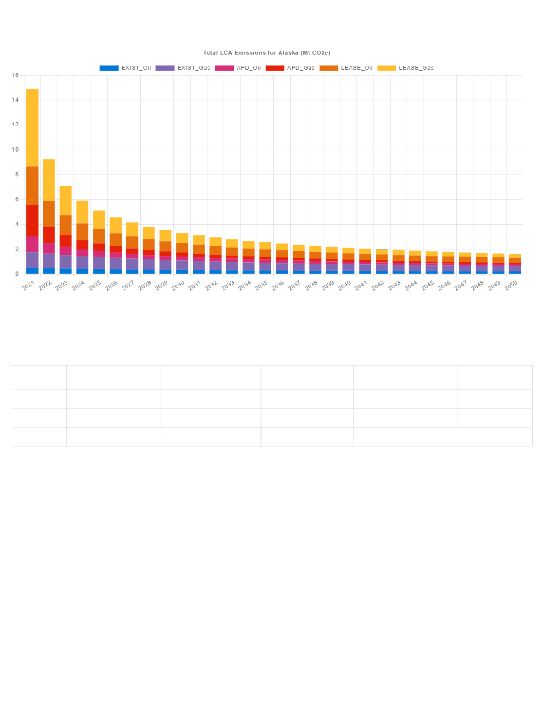
BLM 2021
Figure 5-1 shows an annualized timeline of the projected short-term life-of-project emissions from the tables
above for the selected state. The cumulative sum of all the state series is displayed in Table 5-17.
S t a t e P r o j e c t i o n S e r i e s S u m = 1 0 5 . 4 7 ( M t C O e )
Figure 5-1. State Oil and Gas Emissions Timelines (Alaska)
Table 5-17. Federal Summary - Projected Short-Term Life-of-Project Emissions (Mt)
5.3 Long-Term Federal Fossil Fuel Mineral Emissions Projections
The long-term emissions estimates presented in Figure 5-2 and Table 5-18 are based on 2021 EIA Annual
Energy Outlook (AEO) data. Here the BLM is providing access to all of the AEO cases, as these explore a
variety of market conditions including varying production, price, and overall economic growth rates. The
difference (or delta) between the cumulative short-term emissions previously described and the long-term
emissions estimates can be thought of as the level of additional development that could be authorized to
sustain the existing federal fraction of production over the longer term. Similarly, if the short-term emissions
exceed a longer term scenario, then the delta can be thought of as the amount of reduction required to attain
the outlook forecast. In all cases, the EIA clearly explains that the AEO scenario projections are not
predictions of what will happen, but rather, they are modeled projections of what may happen given certain
assumptions.
For the 2021 AEO, the High Oil Price scenario produces the highest emissions. This should also be true at
subnational scales depending on the production resource mix. However, areas with higher levels of coal
production could see higher emissions even in a Low Oil and Gas supply scenario. For all areas (cumulative),
2
5.6593 0 30.4683 509.92 546.06
225.8 134.56 28.81 1,231.86 1,621.07
221.15 71.54 475.11 1,918.66 2,686.44
Extraction CO2e Processing CO2e Transport CO2e Combustion CO2e Total CO2e
Coal
Oil
Gas
Mineral

BLM 2021
the Low Oil Price case provides the lowest emissions, which is slightly counter intuitive considering that the
Low Renewables Cost case would be expected to produce fewer emissions overall.
Table 5-18. Long-Range Federal Mineral Projections - AEO Reference Case
Onshore federal mineral estate
AEO Total Projected U.S. Production - Reference Case: Coal = 14,449.67 (MM short tons), Oil = 397.24 (MM b/d), Gas =
1,161.80 (Tcf).
The projections made from the 2021 AEO data show that fossil fuel mineral development on federal land
accounts for approximately 13.83% of total U.S. GHG emissions. The difference in federal emissions on an
absolute basis between the High and Low AEO projection scenarios is approximately 2,164.4 Mt of CO e over
the entirety of the projection period, or about 72.15 Mt of CO e on an annual average basis.
* * *
Federal Minerals Federal Production Energy (Quads) Emissions (Mt CO e)
2
Coal (MM short tons) 5,325.36 132.7612 10,151.36
Oil (MM b/d) 24.43 51.6835 5,089.09
Gas (Tcf) 117.71 119.2700 8,871.90
Projected Totals NA 303.71 24,112.35
2
2

BLM 2021
This chapter provides background on cumulative GHG emissions at global, national, and state scales.
Emissions are summarized from the latest global and national inventories for all sources and provide explicit
accounting for GHGs from fossil fuel combustion. The chapter also documents projected emissions of GHGs
at global and national scales. State-level data is provided for select categories of emitters (large sources
and energy related sectors) from the various available databases subsequently described. This information
is useful for providing the cumulative context for which the GHG emissions from BLM’s fossil fuel
authorizations are a part.
6.1 Annual Global Emissions
According to current data from the United Nations Emissions Gap Report (2020), and the Emissions
Database for Global Atmospheric Research (EDGAR), total global GHG emissions grew in 2019 for the third
year in a row and were estimated at 59,100 Mt (59.1 gigatonnes). This represents a 68% increase in global
emissions relative to 1990 levels, a 50% increase over 2010 levels, and a 2.6% increase over the previous
year’s emissions due primarily to a significant increase in wildfires. In addition to increases in total GHG
emissions, increases in CO emissions attributable to fossil fuel use in industrial processes and combustion
(fossil CO ) were also reported. Global fossil CO emissions were estimated at 38,000 Mt for 2019. This
represents an increase in fossil CO emissions of 1.0% over the previous year. To put the magnitude of 2019
global total GHG emissions and fossil CO emissions into perspective, there is general consensus among
climate scientists that to limit global temperature rise to 1.5°C and avoid serious climate changes, global
emissions must drop to 25,000 Mt by 2030 .
Figure 6-1a shows the global fossil CO emissions between 1990 and 2019 and includes predicted emissions
for 2020. Figure 6-1b shows the fossil CO emissions for the largest emitting countries compared to the
remaining countries. In 2019, the world’s 6 largest emitters of fossil CO ; China, the United States, India, the
EU27+UK, Russia and Japan, together accounted for 51% of the population and emitted 67.0% of total global
fossil CO emissions. The largest emitter was China with 11,535 Mt or 30.3% of global CO emissions
followed by the U.S. with 5,107 Mt or 13.4% of the global emissions. The largest increases in emissions over
the previous year were from China (3.4%) and India (1.6%). Decreases in fossil CO emissions were achieved
in the EU27+UK (-3.8%), the United States (-2.6%), Japan (-2.1%), and Russia (-0.8%) . Early estimates of
the impact of the COVID-19 pandemic and resulting economic crisis indicate that global energy related
emissions fell by almost 6% in 2020 as demand for fossil fuels decreased by 4%-9% . However, this
decrease in demand and associated GHG emissions is expected to be short-lived as fossil fuel consumption
is on the rise in 2021.
2
2 2
2
2
[20 ]
2
2
2
2 2
2
[21 ]
[22 ]
6.0 Global, National, and State GHG Emissions
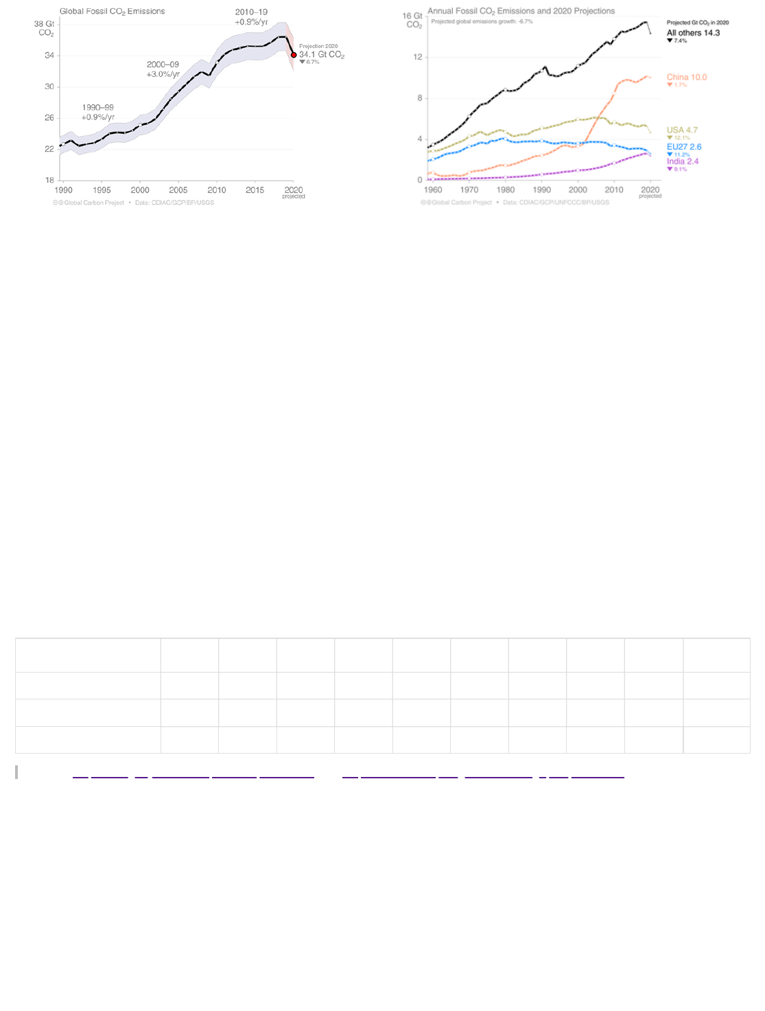
BLM 2021
(a) (b)
Figure 6-1. Global Fossil CO Emissions
Globally, the use of all fossil fuels (coal, oil, gas, and peat), and the CO emissions associated with the
combustion of these fuels, continues to rise. Table 6-1 shows global total GHG emissions and U.S. fossil
CO emissions over the last decade. The U.S. fossil CO emissions as a percent of global total GHG
emissions has averaged nearly 10% during this time. Figure 6-2 shows global and U.S. CO emissions from
fossil fuel consumption between 1960 and 2020 for the three major fossil fuels and cement manufacturing
(which releases CO through chemical processes). The large increases in global coal emissions since 2000
can mostly be attributed to China’s increase in coal fired power plants, while in the U.S. emissions from this
fuel type continue to decline due in part to the competitiveness of natural gas and renewable sources of
energy. CO emissions from global oil combustion have remained steady over the last decade while
emissions from oil in the U.S. increased in recent years due primarily to the increase from new production in
basins such as the Permian and Williston and offshore regions. CO emissions from natural gas have
increased dramatically both globally and, in the U.S., due to increases in production and demand as a
replacement fuel for coal. Table 6-2 shows global and U.S. fossil CO emissions from the combustion of
three fuel types (coal, oil, and gas) and the U.S. share of these emissions between 2010 and the year of most
recent available data (2018).
Table 6-1. Total Global GHG Emissions 2010 – 2019 (Mt/yr)
Source: https://edgar.jrc.ec.europa.eu/report_2020 and https://www.unep.org/emissions-gap-report-2020.
2
2
2 2
2
2
2
2
2
Emissions Scope 2010 2011 2012 2013 2014 2015 2016 2017 2018 2019
Global - Total GHGs 50,100 53,000 54,000 54,700 52,700 52,700 52,800 53,500 55,300 59,100
U.S. - Fossil CO
2
5,568 5,439 5,264 5,337 5,413 5,249 5,153 5,083 5,244 5,107
U.S. Share 11.1% 10.3% 9.7% 9.8% 10.3% 10.0% 9.8% 9.5% 9.5% 8.6%
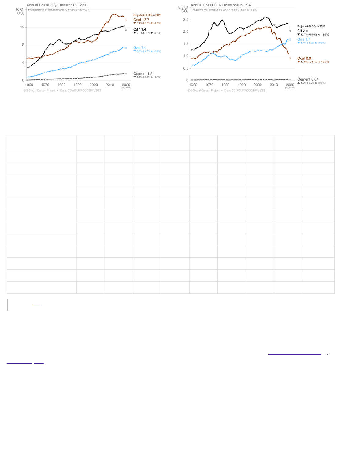
BLM 2021
(a) (b)
Figure 6-2. Annual Fossil Fuel CO Emissions (Global and U.S.)
Table 6-2. Total CO Emissions from Fossil Fuel Combustion (Mt/yr)
Source: IEA https://www.iea.org/data-and-statistics/data-product/co2-emissions-from-fuel-combustion-highlights
All Fuels – includes marine and aviation bunker fuels in addition to coal, oil, and gas.
6.2 Projected Global Emissions
The EIA provides long-term (2018–2050) world energy and emissions projections in its International Energy
Outlook (IEO). The most recent IEO that contains CO emissions data is the IEO2020, released in October
2020. The IEO provides several different scenarios to forecast future energy needs and associated carbon
emissions. The Reference case reflects current trends and relationships among supply, demand, and prices
in the future and is a reasonable baseline case to compare with cases that include alternative assumptions
about the future energy system. Similar to the AEO report, IEO provides a Reference case that assumes
energy consumption will rise nearly 50% between 2018 and 2050. Worldwide coal production and
consumption is assumed to be steady at about 8 billion short tons, while demand for liquid fuels (oil)
increases by 20%, and natural gas consumption increases more that 40% by 2050. Global energy related CO
emissions are projected to increase by 0.6% per year from 2018 to 2050 from about 35 billion metric tons
CO to about 43 billion metric tons. Although aggregate CO emissions from the energy sector are projected
2
2
Emissions Scope 2010 2011 2012 2013 2014 2015 2016 2017 2018
Global - All fuels 30,582 31,459 31,806 32,371 32,389 32,366 32,375 32,837 33,513
U.S. - All fuels 5,352 5,128 4,903 5,039 5,047 4,929 4,838 4,761 4,921
U.S. All Fuels Share 17.5% 16.3% 15.4% 15.6% 15.6% 15.2% 14.9% 14.5% 14.7%
Global - Coal 13,828 14,584 14,714 15,020 14,989 14,607 14,343 14,506 14,766
U.S. - Coal 1,982 1,870 1,648 1,705 1,699 1,465 1,356 1,324 1,270
U.S. Coal Share 14.3% 12.8% 11.2% 11.4% 11.3% 10.0% 9.5% 9.1% 8.6%
Global - Oil 10,554 10,573 10,669 10,838 10,889 11,141 11,228 11,354 11,415
U.S. - Oil 2,060 1,929 1,870 1,926 1,914 1,984 1,992 1,981 2,031
U.S Oil Share 19.5% 18.2% 17.5% 17.8% 17.6% 17.8% 17.7% 17.4% 17.8%
Global - Gas 6,038 6,123 6,239 6,325 6,322 6,427 6,592 6,759 7,104
U.S. - Gas 1,287 1,304 1,361 1,386 1,412 1,459 1,470 1,437 1,601
U.S. Gas Share 21.3% 21.3% 21.8% 21.9% 22.3% 22.7% 22.3% 21.3% 22.5%
2
2
2 2
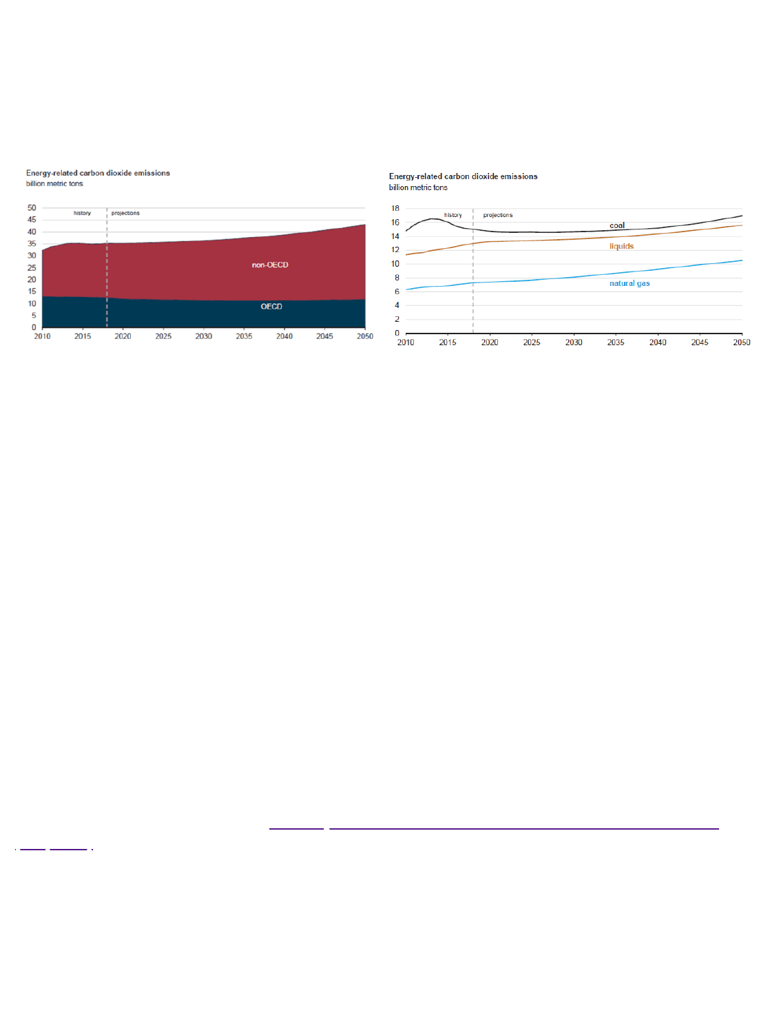
BLM 2021
to continue to rise, the carbon intensity of future energy sources (i.e., the amount of CO emissions produced
per unit of energy used) is projected to decrease indicating that sources of energy that do not produce CO
emissions (e.g., renewables) will comprise a larger portion of meeting future energy demands. Figure 6-3
(EIA graphs) shows both the last decade of estimated CO emissions from global fossil fuel combustion and
the projected emissions out to 2050. The data is displayed separately for countries that are a part of the
Organization of Economic Cooperation and Development (OECD), of which the U.S. is a part, and those that
are not.
(a) (b)
Figure 6-3. Reference Case – Future Global Energy Related CO Emissions
6.3 Annual U.S. Emissions
The U.S. EIA provides information on energy related CO emissions in its Monthly Energy Review (MER). The
January 2021 edition of the MER shows that U.S. energy-related CO emissions fell by an estimated 11%
from 5,140 Mt in 2019 to 4,571 Mt in 2020, largely because of reduced travel and other factors that led to
less energy consumption during the COVID-19 pandemic. Emissions from coal combustion in the U.S.
comprised 19% of the energy consumption emissions while oil and gas consumption accounted for 45% and
36% of emissions, respectively.
The U.S. EPA provides a comprehensive accounting of total GHG emissions for all man-made sources in the
United States. The results of these tracking and quantification efforts are published in the annual Inventory
of U.S. Greenhouse Gas Emissions and Sinks. The inventory report is a top-down assessment of national
annual GHG emissions and is prepared to comply with commitments under the United Nations Framework
Convention on Climate Change (UNFCCC). The EPA generally uses national energy data, data on national
agricultural activities, and other national statistics to provide a comprehensive accounting of total GHG
emissions. The use of the aggregated national data results in total coverage of sources including small
emitters but means that the national emissions estimates for most source categories are not broken down at
the geographic or facility level.
According to the latest version of the Inventory of U.S. Greenhouse Gas Emissions and Sinks: 1990-2019
(EPA, 2021) released in April 2021, total U.S. GHG emissions were 6,558.3 Mt of CO e in 2019, a decrease of
approximately 1.7% from the previous year and a decrease of 13% from the peak emissions in 2005. The
decrease in total GHG emissions between 2018 and 2019 was largely driven by the decrease in CO
emissions from fossil fuel combustion primarily from shifts in the electrical power sector from coal to gas
and other renewables. However, 82% (5,392 Mt) of the total emissions were due to energy production and
use, primarily fossil fuel combustion for transportation and electricity generation. The tonnages presented in
this paragraph were calculated by EPA using GWPs from the IPCC’s AR4. The EPA also presents emissions
estimates using GWPs from IPCC’s AR5 in the Annexes to the Inventory of U.S. GHG Emissions and Sinks.
2
2
2
2
2
2
2
2
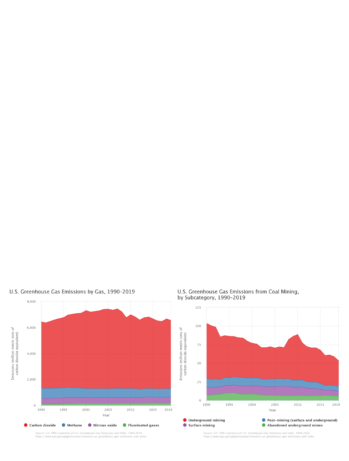
BLM 2021
The primary GHG emitted by human activities in the U.S. was CO , representing approximately 80% of total
2019 GHG emissions. The largest source of CO , and of overall GHG emissions, was fossil fuel combustion
(4,857 Mt). CH emissions from all sectors (673.51 Mt) accounted for 10% of emissions and increased
slightly for the first time since 2011. The major sources of CH include natural gas systems, enteric
fermentation and manure management associated with domestic livestock, and decomposition of wastes in
landfills. N O emissions accounted for 7% of total GHG emissions. The agricultural sector including
fertilizers and soil management and manure management was the largest source of N O emissions. Figure
6-4a shows total U.S. GHG emissions by greenhouse gas.
The EPA GHG inventory report includes emissions data broken out by five different emissions sectors. The
Energy sector includes three different subcategories; coal mining, natural gas and petroleum systems, and
fossil fuel combustion. The emissions itemized under the coal mining and natural gas and petroleum
systems subcategories include emissions for all U.S. sources in each of these categories and are not
differentiated by mineral ownership (i.e., federal, state, or private minerals). The coal mining sector includes
emissions from underground and surface mining as well as post mining activities and abandoned
underground mines. In 2019, GHG emissions from this subcategory were 53.31 Mt a decrease of 9.5% from
the previous year. Figure 6-4b shows a dramatic decrease in coal mining emissions since 2010 and an
overall decrease in emissions of 49% since 1990 from this subcategory.
The natural gas and petroleum systems subcategory includes emissions from oil and gas exploration,
production, and processing as well as other sources. In 2019, GHG emissions from this subcategory were
287.83 Mt, an increase of 7.3% from the previous year. Figure 6-4c shows a steady increase in emissions
from this subcategory since the low point in 2016, but overall emissions have remained fairly steady since
1990 with an overall increase of 1.2% from this subcategory.
The fossil fuel combustion subcategory includes emissions from use of fossil fuels in transportation,
electricity generation, industry, and residential use. In 2019, emissions from this subcategory were 4,856.7
Mt, down 2.7% from the previous year and down 15.6% from the peak in 2007. Figure 6-4d shows the CO
emissions from fossil fuel combustion since 1990.
(a) (b)
2
2
4
4
2
2
2
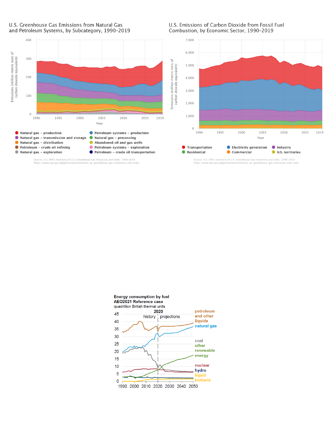
BLM 2021
(c) (d)
Figure 6-4. U.S. GHG Emissions
6.4 Projected U.S. Emissions
In addition to providing long-term projections for global energy demand and associated CO emissions, the
EIA produces an assessment of domestic energy and emissions trends through 2050 in its AEO report (as
discussed in chapter 4). The AEO projections for energy-related CO emissions from fossil fuel consumption
generally show a slight decrease in emissions over the next decade due primarily to significant decreases in
coal consumption and a rise in the use of natural gas and renewable energy sources to meet demand.
However, U.S. CO emissions from energy consumption are expected to increase beyond 2035 due to
increases in population and economic growth and the associated increases in oil and natural gas
consumption. Figure 6-5 shows the projected changes in U.S. fossil fuel use through 2050.
Figure 6-5. U.S. Projected Energy Mix (2021 AEO)
6.5 State Emissions
2
2
2

BLM 2021
Each year, the U.S. EPA and the EIA compile data on GHG emissions at the state level as well as nationally.
The EPA collects detailed emissions data from the largest greenhouse gas emitting facilities in the U.S.
through its GHG Reporting Program (GHGRP). Large emitters of GHG emissions (> 25,000 tons/year) in each
state are required to report their annual emissions along with other relevant facility data. Approximately
8,000 facilities report their emissions annually. The data is compiled by facility and by state and are
available through EPA’s Facility Level Information on GreenHouse gases Tool (FLIGHT). The GHGRP data are
useful for understanding the major sources and types of GHG emissions within a state; however, it is not a
comprehensive emissions inventory for each state as many sources of emissions (e.g., agriculture and land
use sectors) are not required to report. The EPA has estimated that GHGRP reporting covers approximately
85% of the total GHG emissions for sector-specific sources. The EIA issues its State Energy-Related Carbon
Dioxide Emissions Tables on an annual basis that show CO emissions from fossil fuel use for sources
across all sectors of the economy (residential, commercial, industrial, transportation, and electricity
generation). Table 6-3 shows GHG emissions as reported to EPA for the states in which the BLM authorizes
leasing and development of federal fossil fuel minerals. Information is shown for total reported GHG
emissions from all facilities in each state as well as for two subcategories; power plants that consume coal
or natural gas, and petroleum and natural gas systems that produce or consume oil or gas. The table also
shows CO emissions from the combustion of fossil fuels in each state as estimated by EIA.
2
2

BLM 2021
Table 6-3. State GHG Emissions (Mt/yr CO )
EPA FLIGHT data (large emitters), and EIA State Energy related CO emissions data.
EPA and EIA state emissions data does not include emissions from agriculture or waste management.
* * *
2
80.9 51.6 2.3 113.4
14.4 3.1 8.5 35.2
41.8 33 0.4 71.4
93.2 31.2 5.7 362.5
45.3 34.3 4.3 89.3
5.1 1.7 0.3 19
96.4 59.4 1.8 210.2
34.1 20.5 2.2 62.4
78.4 58.7 1.1 120.7
146.3 40.1 22.8 210.8
79.5 56.5 2.2 162.1
39.8 25.2 1.9 69.4
20.9 16.4 0.9 30.7
28.9 21 0.4 52.7
17.1 13.8 0.3 37.9
29.7 21.4 5 45.4
34.5 23.6 2 167.5
37.8 28.2 2.4 59.2
104.6 67.2 3.3 208.6
51.4 28.4 4.5 97.9
114.5 77.3 3.5 221.3
6.4 3.3 0 15.6
380.5 203.4 30.9 701.1
36 28 0.9 60.3
42.6 27.5 0.6 103.1
74.7 56.5 2 89.9
54.5 39.1 5.2 63.6
2
EPA GHGRP
Total Reported
EPA GHGRP
Power Plants
EPA GHGRP Petroleum
& Natural Gas Systems
EIA Energy Related
Emissions
Alabama
Alaska
Arkansas
California
Colorado
Idaho
Illinois
Kansas
Kentucky
Louisiana
Michigan
Mississippi
Montana
Nebraska
Nevada
New Mexico
New York
North Dakota
Ohio
Oklahoma
Pennsylvania
South Dakota
Texas
Utah
Virginia
West Virginia
Wyoming
State

BLM 2021
For the purposes of NEPA analyses, the BLM uses the decision scope emissions (i.e., reasonably foreseeable
GHG emissions) of a proposed federal action as a proxy for assessing climate impacts. Published climate
impact predictions associated with various global emissions scenarios are described in the NEPA analysis
and are compared to the decision scope emissions levels to provide a basis for considering the magnitude,
or range of impacts, that could follow from the proposed action. This methodology for assessing climate-
related impacts is in line with previously issued guidance and has obvious benefits in that emissions
calculations are relatively straightforward and can be clearly explained if properly documented. More
specifically, the proxy approach was adopted because of the lack of climate analysis tools and techniques
that lend themselves to describing the physical climate or earth system responses, such as changes to sea
level, average surface temperatures, or regional precipitation rates, that could be attributable to emissions
associated with any single action or decision. Comparing proxy emissions at various scales relative to a
quantity of emissions known to have a definitive climate impact (i.e., modelled emissions) allows the BLM to
provide a clearly understandable sense of the intensity for an action relative to the magnitude of the issue.
Further, there are no established emissions thresholds for NEPA analysis to contextualize the quantifiable
GHG emissions of an action or decision in terms of environmental effects. Although future policy may
prescribe an emissions threshold for analysis, the implications of such a limit (physical or otherwise) are
beyond the scope of this report to contemplate presently. One of the drawbacks of the proxy emissions
method is the difficulty in downscaling the published climate impacts (predicted or observed) relative to the
federal action emissions, which are typically several orders of magnitude smaller than the emissions levels
associated with the published impacts. Still, comparing emissions levels between proposed actions, current
emissions and conditions, and published predictions based on forecasted emission scenarios allows
decisionmakers to form a qualitative judgment about the potential for climate impacts from a proposed
action.
7.1 Emissions Comparisons
The annual global and U.S. emissions data presented in chapter 6 can be compared with the estimated
annual GHG emissions from BLM fossil fuel authorizations in chapter 5 to provide context around the scale
and potential impact of estimated emissions from BLM’s fossil fuel authorizations. Evaluating the magnitude
of estimated emissions from a particular category in the context of other categories or total geographic
emissions is one way to evaluate their relative potential impact on climate change. A comparative analysis is
also useful for informing policy and planning decisions and to identify options for maximizing the
effectiveness of mitigation and emissions reduction strategies. Table 7-1 compares the magnitude of BLM’s
estimated emissions to global and U.S. emissions at different scales. For example, the table shows that the
emissions associated with the BLM's authorizing of leasing and extraction of federal minerals on public
lands, (i.e., direct emissions from coal, oil, and gas) comprise 0.09% of global emissions and 0.8% of U.S.
emissions. The total emissions from coal, oil, and gas development and end-use comprise 1.6% of global
emissions and 14.0% of U.S. emissions. It is important to note that the U.S. emissions shown in the table
(U.S. total, energy production, fossil fuel combustion, coal mining, and natural gas and petroleum systems)
are derived using GWPs from IPCC AR4 to convert to CO equivalents, whereas BLM emissions are derived
using GWPs from IPCC AR5 (see Table 3-1). This may result in a slight overestimation of BLM’s share of U.S.
emissions in the table.
[23 ]
2
7.0 Emissions Analysis

BLM 2021
Table 7-1. BLM Share of 2019 Annual Global and U.S. GHG Emissions
Not applicable "NA" cells are irrelevant to calculated data columns.
Table 7-2 presents emissions data for large emitters and energy-related CO emissions for the states in
which the BLM has authorized leasing and development of federal fossil fuel minerals. The annual emissions
data from the EPA and EIA (see Chap. 6) are compared to the BLM’s estimated annual direct emissions in
each state for the report year. The BLM-authorized direct emissions are used for comparison rather than
total emissions, because the direct emissions reflect the portion of emissions known to occur in that state.
Emissions from processing, transport, and downstream combustion (indirect) may or may not occur in the
state where the minerals were first extracted. Although the BLM has attributed indirect emissions to the
state where the minerals are extracted for accounting purposes in Chapter 5 of this report, that approach is
not valid for state-level comparison purposes in this chapter. For example, more than 80% of the coal
extracted from federal minerals in Wyoming is transported and combusted outside of Wyoming. If the total
BLM-authorized emissions (direct and indirect) in Wyoming were compared to EPA FLIGHT data and EIA state
data for Wyoming, it would appear that BLM emissions in Wyoming comprised 912% of Wyoming’s large
emitters and 782% of Wyoming’s energy-related CO emissions. This is nonsensical, so a comparison of
total emissions at the state scale is not valid. Total emissions are compared to global and national
emissions in Table 7-1. Instead, Table 7-2 shows that the BLM’s direct emissions in Wyoming are equivalent
to 26% of emissions from large emitters in Wyoming and equivalent to 23% of energy-related emissions in
Emissions Category
Annual
Emissions
(Mt)
BLM Share
Total
Emissions
All fuels
Indirect
Emissions
All Fuels
Direct
Emissions
All Fuels
Direct
Emissions
Oil and
Gas
Direct
Emissions
Coal
Mining
Global - Total GHG Emissions 59,100.00 1.6% 1.5% 0.09% 0.1% 0.0%
Global - Fossil Fuel Combustion 33,513.25 2.7% 2.6% 0.15% 0.1% 0.0%
U.S. Total GHG Emissions 6,558.30 14% 13.2% 0.8% 0.7% 0.1%
U.S. Energy Production 5,392.27 17% 16.1% 0.9% 0.8% 0.1%
U.S. Fossil Fuel Combustion 4,856.70 18.9% 17.9% 1.0% 0.9% 0.1%
U.S. Coal Mining 53.31 NA NA NA NA 9.1%
U.S. Natural Gas
and Petroleum Systems
287.83 NA NA NA 15.8% NA
BLM Total GHGs from
all Fossil Fuel Authorizations
918.64 100% 94.5% 5.5% 4.9% 0.5%
BLM Indirect GHG Emissions
from all Fossil Fuel Authorizations
868.36 NA 100% NA NA NA
BLM Direct GHG Emissions from
all Fossil Fuel Authorizations
50.28 NA NA 100% 90.4% 9.6%
BLM Direct GHG Emissions from
Oil and Gas Authorizations
45.43 NA NA NA 100% NA
BLM Direct GHG Emissions from
Coal Authorizations
4.85 NA NA NA NA 100%
2
2

BLM 2021
Wyoming. This example illustrates that it is valid to compare BLM total emissions at U.S. and global scales
and to compare BLM direct emissions at the state scale.
Table 7-2. BLM Share of State Annual GHG Emissions (MMT CO )
2
0.1 80.9 0.1% 113.4 0.1%
0.19 14.4 1.3% 35.2 0.5%
0.05 41.8 0.1% 71.4 0.1%
0.8 93.2 0.9% 362.5 0.2%
4.75 45.3 10.5% 89.3 5.3%
<0.001 5.1 0% 19 0%
<0.001 96.4 0% 210.2 0%
0.03 34.1 0.1% 62.4 0.05%
<0.001 78.4 0% 120.7 0%
0.21 146.3 0.1% 210.8 0.1%
0.01 79.5 0% 162.1 0.005%
0.02 39.8 0% 69.4 0.03%
0.49 20.9 2.4% 30.7 1.6%
<0.001 28.9 0% 52.7 0%
0.02 17.1 0.1% 37.9 0.1%
23.37 29.7 78.7% 45.4 51.4%
<0.001 34.5 0% 167.5 0%
3.69 37.8 9.8% 59.2 6.2%
0.02 104.6 0% 208.6 0.01%
0.16 51.4 0.3% 97.9 0.2%
<0.001 114.5 0% 221.3 0%
0.01 6.4 0.2% 15.6 0.1%
0.16 380.5 0% 701.1 0.02%
1.69 36 4.7% 60.3 2.8%
<0.001 42.6 0% 103.1 0%
<0.001 74.7 0% 89.9 0%
14.5 54.5 26.6% 63.6 23%
BLM Fossil Fuel
Authorizations
Direct
Emissions
EPA GHGRP
Large
Emitters
BLM Share of
Large
Emitters
EIA Energy
Related
Emissions
BLM Share of Energy
Related Emissions
Alabama
Alaska
Arkansas
California
Colorado
Idaho
Illinois
Kansas
Kentucky
Louisiana
Michigan
Mississippi
Montana
Nebraska
Nevada
New Mexico
New York
North Dakota
Ohio
Oklahoma
Pennsylvania
South Dakota
Texas
Utah
Virginia
West Virginia
Wyoming
State

BLM 2021
7.2 Carbon Budgets and Carbon Neutrality
Carbon neutrality, or net zero emissions, is maintaining a balance between emitting and absorbing GHGs
from the atmosphere. On a global scale, carbon neutrality would result in atmospheric concentrations of
GHGs reaching an equilibrium, which could stabilize climate change and limit global warming. Under the
2015 Paris Agreement, countries agreed to cut GHG emissions with the goal of holding the increase in the
global average temperature to well below 2°C above pre-industrial levels and pursuing efforts to limit the
temperature increase to 1.5°C above pre-industrial levels in order to avoid some of the more dire
consequences associated with climate change. Carbon budgets are an estimate of the amount of additional
GHGs that could be emitted into the atmosphere over time to reach carbon neutrality while still limiting
global temperatures to no more than 1.5°C or 2°C above pre-industrial levels. At the time of this draft, the
IPCC Special Report on Global Warming of 1.5ºC (2018) is the most widely accepted authority on the
development of a carbon budget to meet the goals of the Paris Agreement. Other organizations have also
developed carbon budgets for specific sectors and emissions and temperature targets. For example, the
International Energy Agency (IEA) developed its carbon budget focused on the energy sector in its report on
achieving Net Zero by 2050. The International Renewable Energy Agency (IRENA) developed a carbon budget
focused on rapid transition from fossil fuels for its Renewables Energy Outlook and its World Energy
Transitions Outlook.
Carbon budgets are dependent on the key assumptions and parameters used to develop the budget such as
source sectors for emissions, GHGs included, temperature targets, climate sensitivity, and estimates of
cumulative carbon emissions that have already occurred. For example, scientists recently revised the IPCC
budget to account for problems associated with the Earth System Models used in the AR5 budget
estimates . These models underestimated historical cumulative CO emissions and were projecting
temperatures warmer than have been observed. The new estimates rely on observational constraints to
make the budget calculations, which have been widely accepted by climate scientists as being more
accurate.
Carbon budget estimates are expressed as the remaining cumulative CO emissions from a base year (most
recently 2018) until the time when net zero global emissions can be achieved. The IPCC budget suggests a
range of approximately 420 GtCO for a 66% chance of limiting warming to 1.5°C to 840 GtCO2 for a 33%
chance. Similarly, estimates for the 2°C probabilities range from 1,170 to 2,030 GtCO . These estimates
contain uncertainties that are characteristic of scientists' current understanding of the Earth's climate
influencing systems, such as feedbacks and the forcing and response associated with the non-CO GHG
species, and historical emissions accounting. The uncertainty range associated with the new estimates is
approximately ±400 Gt CO . Because the IEA and IRENA derived carbon budgets fall within this range of
uncertainty, the BLM primarily discusses the IPCC budgets in this report. Staying within the 1.5°C carbon
budget implies that CO emissions need to start declining this decade to maintain reasonable progress to
reach net zero by about 2050, or 2100 for the 2°C budget. Figure 7-1 outlines what an emissions reduction
curve under either scenario might look like. Note: The 1.5°C pathway to neutrality assumes a higher degree
of emissions reduction than pledges made under the Paris Agreement.
[24 ]
2
2
2
2
2
2
2
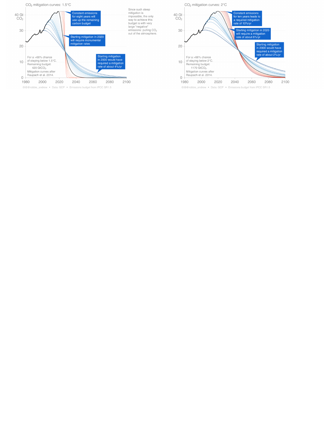
BLM 2021
(a) (b)
Figure 7-1. Carbon Budget Mitigation Pathways
Annually, the United Nations (UN) publishes an emissions gap report which provides an assessment of how
actions and pledges of countries affect global GHG emissions trends and how these trends compare to
emissions trajectories that are consistent with long-term goals for limiting global warming (UN 2020).
Specifically, the emissions gap is the difference between GHG emissions levels consistent with limiting
global warming to 1.5°C or 2.0°C and the emissions levels consistent with current reduction commitments by
member nations. By 2030, the UN estimates that to limit warming to 2.0°C or 1.5°C, global annual emissions
should be approximately 41 GtCO e and 25 GtCO e, respectively. Based on current emissions pledges, the
global emissions gap in 2030 would be 15 GtCO e above the 2.0°C warming goal and 32 GtCO e above the
1.5°C warming goal. To bridge the gap, nations must implement policies to strengthen emissions reductions
commitments threefold to achieve the 2.0°C goal and fivefold to achieve the 1.5°C goal. Delaying the
implementation of stronger policies would require even more stringent emissions reduction policies to
achieve warming goals.
The IEA "Net Zero by 2050" report found that current global emissions commitments fall short of those
needed to limit global warming to 1.5 ºC above pre-industrial levels. The IEA identifies a narrow pathway that
reaches global net-zero emissions by 2050 and limits warming to 1.5 ºC, but it requires countries to
strengthen and successfully implement energy and climate policies. This emissions pathway requires clean
energy investment, innovation to bring new clean energy technologies to market, a shift away from
technology that uses fossil fuels, a focus on transitioning people’s behavior and jobs for a new energy sector,
and international cooperation. Under this emissions pathway, fossil fuel use in the energy sector would fall
from four-fifths of all supply to one-fifth by the year 2050. While the IEA identified a global pathway, each
country needs to design its own strategy for achieving carbon neutrality.
Executive Order 14008, "Tackling the Climate Crisis at Home and Abroad" (January 27, 2021), directs the
executive branch to establish policies or rules that put the United States on a path to achieve carbon
neutrality, economy-wide, by no later than 2050. This goal is consistent with IPCC’s recommendation to
reduce net annual global CO emissions between 2020 and 2030 in order to reach carbon neutrality by mid-
century. Since the EO was issued earlier in 2021, federal agencies are still in the process of developing
policies that align with a goal of carbon neutrality by 2050.
None of the global carbon budgets are a hard line that countries have committed to stay within as part of the
Paris Agreement or otherwise. Carbon budgets were originally envisioned as being a convenient tool to
simplify communication of a complex issue and to assist policymakers considering options for reducing GHG
emissions on a national and global scale. Carbon budgets have not yet been established on a national or
subnational scale, primarily due to the lack of consensus on how to allocate the global budget to each nation,
2 2
2 2
2

BLM 2021
and as such the global budgets that limit warming to 1.5 ºC or 2.0 ºC are not useful for BLM decisionmaking
as it is unclear what portion of the budget applies to emissions occurring in the United States. However,
stakeholders and members of the public have requested that the BLM consider comparing its predicted
emissions in the context of global carbon budgets.
Table 7-3 provides an estimate of the potential emissions associated with BLMs fossil fuel authorizations in
relation to IPCC carbon budgets. The BLM projected life-of-project emissions from existing and foreseeable
federal fossil fuel (oil, gas, and coal) development (see Chapter 5) are used here for the carbon budget
analysis. Oil and gas projected life-of-project emissions are scaled (i.e., time to exhaust budget ÷ 30-year life
of project) to the timeframe in which global emissions will exhaust the budget in order to show the portion of
the budget that is consumed by federal emissions. Since foreseeable federal coal emissions are only
projected for 1 year, it is assumed that the projected 2021 annual federal coal emissions will continue for the
entire timeframe in which budgets are exhausted. This is likely an overestimate since coal reserves on
federal lease tracts will be depleted over time. The BLM estimated emissions include direct emissions as
well as transport and downstream combustion emissions. It is important to note that this comparison of
BLMs estimated emissions from fossil fuel authorizations to global carbon budgets does not portray the full
picture of carbon flux (amount emitted vs. amount stored/sequestered/offset) on public lands. Results of
the carbon budget analysis are presented as the percent of the budget consumed by federal fossil fuel
emissions and the difference in time it takes to consume the budget with and without federal fossil fuel
emissions. The results in the table reflect only the emissions side of the equation and may overestimate
actual consumption of global carbon budgets resulting from BLM leases and authorizations. The U.S.
Geological Survey estimated that sequestration on federal lands offset approximately 15% of CO emissions
resulting from the extraction and end-use combustion emissions of fossil fuels on federal lands. In future
annual iterations of this report, the BLM may refine this carbon budget evaluation based on new or improved
emissions and sequestration information on public lands, and on potential future U.S. policies establishing
carbon neutral emissions pathways.
2
BLM 2021
Table 7-3. Evaluation of Potential Federal Fossil Fuel GHG Emissions with Respect to Global Carbon
Budgets
Based on Long-term Onshore Federal Mineral Emissions estimated from the EIA AEO reference case energy projection
scenario. Does not include sequestration by federal lands or other federal emissions offsets.
Based on the global emissions from the 2020 UN Emissions Gap Assessment, 59.1 Gt CO e.
7.3 Climate Impact Modeling
To move beyond the emissions as a proxy approach for ascribing climate impact attribution as a result of
BLM-authorized emissions, the Bureau has been investigating the use of reduced complexity climate models
to analyze such emissions for the purposes of obtaining actual earth system responses that could be
attributable to the federal decision scope over which the BLM has purview. Most simple climate models are
based in part on global average energy-balance equations, and a few incorporate additional processing
modules to better account for some of the more complex feedback mechanics. The Model for the
Assessment of Greenhouse Gas Induced Climate Change (MAGICC) stands out as a potential resource due to
its ease of use (online access), flexibility, robustness, and overall transparency. As described on the model's
wiki page, "MAGICC is designed to provide maximum flexibility in order to match different types of responses
seen in more sophisticated models, the approach in MAGICC's model development has always been to derive
the simple equations as much as possible from key physical and biological processes." This process-based
approach has a strong conceptual advantage in comparison to simple statistical fits that are more likely to
quickly degrade when emulating scenarios outside the original calibration space of the sophisticated
models. From a user's perspective, the platform offers detailed documentation and baseline scenario
emissions input files that are easily modified to suit the BLM's needs. Figure 7-2 shows MAGICC's
conceptual model workflow.
Carbon Budget (GtCO )
2
840 580 420 2,030 1,500 1,170
14.21 9.81 7.11 34.35 25.38 19.8
Federal Emissions During Budget Timeframe (GtCO )
2
4.67 3.15 2.24 11.68 8.55 6.58
0.56% 0.54% 0.53% 0.58% 0.57% 0.56%
14.29 9.87 7.14 34.55 25.53 19.91
-29 -20 -14 -73 -53 -41
Federal Emissions During Budget Timeframe (GtCO )
2
7.39 5.30 3.91 16.5 12.39 9.97
0.88% 0.91% 0.93% 0.81% 0.83% 0.85%
14.34 9.90 7.17 34.63 25.59 19.97
-46 -33 -24 -103 -77 -62
Federal Emissions During Budget Timeframe (GtCO )
2
12.05 8.44 6.16 28.18 20.94 16.55
1.44% 1.46% 1.47% 1.39% 1.40% 1.41%
14.42 9.96 7.21 34.83 25.74 20.08
-75 -53 -38 -175 -130 -103
1
2
2
Metric
1.5 Deg C 2.0 Deg C
Time to Exhaust Budget (years)
2
Federal
Oil and Gas
Federal Consumption of Budget (%)
Time to Exhaust Budget without Federal Emissions (years)
Reduction in Time to Exhaust Budget from Federal Emissions (days)
Federal Coal
Federal Consumption of Budget (%)
Time to Exhaust Budget without Federal Emissions (years)
Reduction in Time to Exhaust Budget from Federal Emissions (days)
Federal Oil,
Gas & Coal
Federal Consumption of Budget (%)
Time to Exhaust Budget without Federal Emissions (years)
Reduction in Time to Exhaust Budget from Federal Emissions (days)
Minerals
1
33%
50% 66% 33% 50% 66%
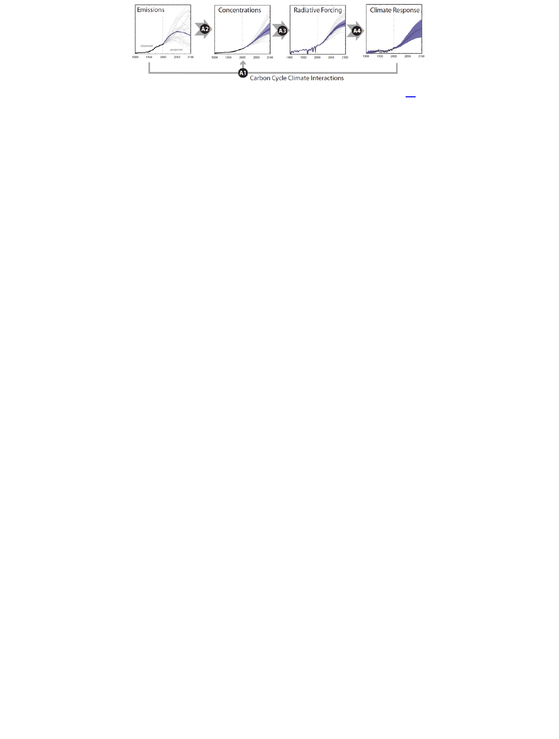
BLM 2021
Figure 7-2. MAGICC Model Calculation Workflow
The BLM has constructed a single run of MAGICC utilizing the 2.6 Representative Concentration Pathway
emissions scenario (discussed further in Chapter 9). Run emissions were prepared by subtracting federal
fossil fuel emissions of CO (as GtC) from the baseline scenario emissions over the available projection
period (2020 to 2050). For the initial federal run, emissions projections were made utilizing the Reference
Case from the 2019 AEO report. All other scenario years and pollutant species remained unchanged from
their baseline values. The 2.6 scenario was chosen for initial analysis because the federal emissions would
have the largest signal (i.e., percent) relative to the other scenarios, each of which have far greater
emissions. The results of the initial MAGICC run suggest that 30-plus years of projected federal emissions
would raise average global surface temperatures by approximately 0.0158 °C., or 1% of the lower carbon
budget temperature target.
* * *
[25 ]
2

BLM 2021
8.1 Introduction to Climate Science
Climate refers to atmospheric conditions (e.g., temperature, humidity, pressure, precipitation, solar radiation,
wind) at a particular location averaged over a long period of time. Climatologists commonly use 30-year
averages of variables, such as temperature and precipitation, as benchmarks for historical comparison and
climate change assessment.
In addition to characterizing long-term weather, climate reflects the frequency, variability, and extreme ranges
of atmospheric variables and phenomena. There are numerous sources of natural climate variability on
scales ranging from years to millennia, including volcanic eruptions (e.g., Robock 2000) , fluctuating solar
irradiance (e.g., Schmidt et al. 2012), and changes to earth’s orbit (Milankovitch cycles). There are also
many “ ” such as the El Niño Southern Oscillation (ENSO), North Atlantic Oscillation, and
Pacific Decadal Oscillation that shape interannual, interdecadal, and multidecadal climate variability. Each of
these sources of natural climate variability occur on distinct time scales, some episodic like volcanic
eruptions, while teleconnections are cyclical with varying periodicities. Moreover, each source of climate
variability produces differing impacts based on region and time of year. For instance, ENSO impacts are
more pronounced during winter in the United States, with a strong Pacific Northwest and southwestern
United States signal, but no clear impact in the central Rocky Mountains. Teleconnections also do not
necessarily produce similar impacts during each occurrence with climate anomalies that differ from typical
patterns associated with specific phases of each teleconnection commonly observed. A notable example is
the 2015-16 El Niño, which was exceptionally dry in California and relatively wet in the Pacific Northwest,
counter to seasonal outlooks and typical El Niño conditions (Cash and Burls 2019) . Multiple modes of
atmospheric and oceanic variability introduce tremendous uncertainty in earth’s climate on interannual to
interdecadal time scales. On longer time scales, GHG concentrations exert a larger influence on earth’s
climate than the higher frequency oscillations that produce natural interannual to multiyear variability.
Because GHG emissions dominate other sources of climate variability on the multidecade to century time
scale, climate change models can project future states of Earth’s climate based on GHG emissions
scenarios.
The American Meteorological Society defines climate change as “any systematic fluctuation in the long-term
statistics of climate elements (e.g., temperature, pressure, or wind) that is sustained over several decades or
longer” (AMS 2012) . While climate has changed throughout earth’s history due to natural forcing, recent
climate change is almost entirely the result of increasing GHG concentrations resulting from human activity
since the Industrial Revolution.
8.2 Climate Forcing and Feedbacks
The driver for the buildup of heat within the climate system is best described in terms of radiative forcing
(RF). The term describes the energy balance (i.e., equilibrium), or the difference between solar radiation
absorbed by the Earth and the energy radiated back to space that will occur given the heliophysics of the
sun-earth system and the basic laws of thermodynamics. Radiative forcing, given in units of watts per
square meter (W m ), has both positive (+ heating) and negative (- cooling) components, such that altering
any of these components will likely cause the climate system to settle into a new equilibrium. GHGs help to
contain solar energy loss by trapping longer wave (low energy) radiation emitted from Earth's surface, and
[26 ]
[27 ]
teleconnections
[28 ]
[29 ]
–2
8.0 Climate Change Science and Trends

BLM 2021
thus act as a positive forcing component for which the buildup of these gases has contributed to the current
changing state of the climate equilibrium towards warming.
Current ongoing global climate change is caused, in large part, by the atmospheric buildup of GHGs, which
may persist for decades or even centuries. The buildup of GHGs such as CO , CH , N O, and fluorinated
gases since the Industrial Revolution (1760 to 1840) has substantially increased atmospheric concentrations
of these compounds compared to background levels. Several types of activities contribute to the
phenomenon of climate change, including emissions of GHGs (especially CO and CH ) from fossil fuel
development, large wildfires, activities using combustion engines, changes to the natural carbon cycle, and
changes to radiative forces and reflectivity ( ). It is important to note that GHGs will have a sustained
climatic impact over different temporal scales due to their differences in warming potential and atmospheric
lifespans.
Between 1750 and 2011, cumulative anthropogenic CO emissions emitted to the atmosphere were
approximately 2,040 ± 310 GtCO . About 43% of these emissions have remained in the atmosphere (880 ± 35
GtCO ), while the rest was removed from the atmosphere and stored in natural terrestrial ecosystems (plants
and soils – 29%) and in the oceans (28%). Although CO levels in the atmosphere have varied perpetually
throughout Earth’s history along with corresponding variations in climatic conditions, industrialization and
the burning of carbon-based fossil fuel sources have caused CO concentrations to increase measurably,
from approximately 280 ppm in 1750 to 413.67 ppm as of March 2020. The rate of increase in CO is
unprecedented, at more than 250 times faster than from natural sources after the last Ice Age (NASA 2021)
. This fact is demonstrated by data from the Mauna Loa CO monitor in Hawaii that documents
atmospheric concentrations of CO going back to 1960, at which point the average annual concentration was
recorded at approximately 317 ppm. The record shows that approximately 72% of the increase in
atmospheric CO concentration since pre-industrial times (1750) occurred within the last 60 years. The
Mauna Loa site also contains updated trend data for CH and N O (see Figure 8-1). The trends correspond
to an increasing population and rising standards of living and modernization around the globe.
From pre-industrial times to present, emissions from fossil fuel combustion and cement production have
released 375 [345 to 405] GtC to the atmosphere (68%), while deforestation and other land use change are
estimated to have released 180 [100 to 260] GtC (32%). Concentrations of CO , CH , and N O are now
substantially higher than concentrations found in various ice cores dating back to the past 800,000 years.
Table 8-1 shows a summary of the anthropogenic changes to atmospheric GHGs since pre-industrial times.
The estimated concentrations of CH have more than doubled (722 ppb to 1,874 ppb), while N O
concentrations have increased by a fifth (270 ppb to 333 ppb).
2 4 2
2 4
albedo
2
2
2
2
2
2
[30 ]
2
2
2
4 2
2 4 2
4 2
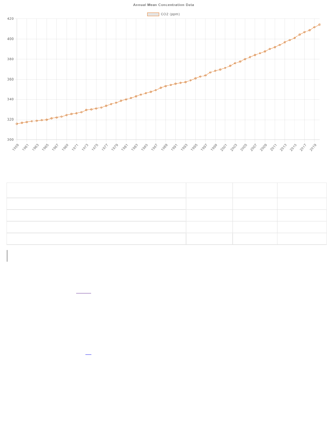
BLM 2021
Figure 8-1. Atmospheric GHG Concentrations
Table 8-1. Global Atmospheric Concentration and Rate of Change of Greenhouse Gases
Source: https://gml.noaa.gov
ppm = parts per million, ppb = parts per billion.
Each year, the National Oceanic and Atmospheric Administration (NOAA) publishes updates to its Annual
Greenhouse Gas Index (AGGI). The AGGI was developed to provide an easily understood standard for
expressing the climate-warming influence of long-lived GHGs. Specifically, the AGGI is the ratio of the total
direct climate forcing from measured long-lived GHG concentrations compared to the 1990 baseline year
(chosen because it is the baseline year for the Kyoto Protocol and the publication year of the first IPCC
Scientific Assessment of Climate Change).
The 1990 baseline year is given an AGGI value of 1.0, and the pre-industrial era is given a value of 0.0 (see
Figure 8-2) (Lindsey 2020) . The AGGI for 2020 was 1.47 which corresponds to CO equivalents
atmospheric concentration of 504 ppm. This represents a 45% increase to climate forcing since 1990 and a
1.8% increase over 2018 levels. While the AGGI does not predict the amount the Earth’s climate has warmed,
it does provide a measure of the effect of GHG emissions on the climate system.
GHG Metric CO (ppm) CH (ppb) N O (ppb)
2 4 2
Pre-Industrial Concentration 278 722 270
2020 Atmospheric Concentration 414.2 1,879.3 333
2020 Concentration Relative to Pre-Industrial 149% 260% 123%
Rate of Change over last 10 years (ppm|ppb/yr) 2.39 8.1 0.96
[31 ]
2
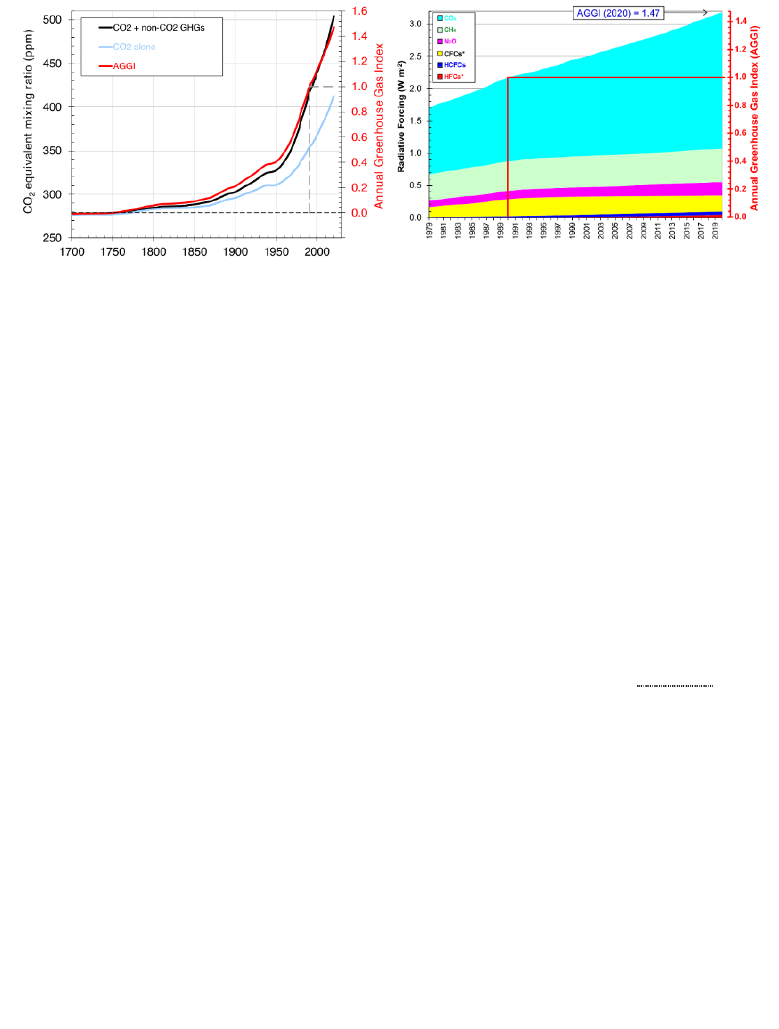
BLM 2021
(a) (b)
Figure 8-2. 2020 Annual GHG Index
The total anthropogenic RF for 2011 relative to 1750 (i.e., the pre-industrial era) was 2.29 ± 1.04 W m ,
which includes both heating and cooling parameter estimates. For well-mixed GHGs, the total positive
forcing is estimated to be 2.83 ± 0.29 W m . The largest contribution to total RF since 1750 is caused by
the increase in the atmospheric concentration of CO . Emissions of CO alone caused an RF of 1.82 ± 0.19
W m (64%), while CH caused an RF of 0.48 ± 0.05 W m (17%). The data highlights methane’s important
role as a potent greenhouse gas, given its RF value in relation to its atmospheric loading trend, approximately
556 Tg yr−1 (64% anthropogenic, 36% natural), and relatively short atmospheric lifetime (12 years). N O has
the third largest forcing of the anthropogenic gases, at 0.17 ± 0.03 W m (6%). Collectively, the three GHGs
of concern account for approximately 87% of the positive forcing within the climate system.
Earth's climate system is complex and interwoven in ways that are not yet fully understood. There are
several known climate feedback mechanisms that add uncertainty in terms of timing (fast and slow
feedbacks) and overall sensitivity within the evaluation of the climate system. Sensitivity refers to the
amount of positive or negative feedback that occurs in response to a given forcing. The feedbacks and
processes connecting RF to a climate response can operate on a large range of time scales. Reaching
temperature equilibrium in response to anthropogenic activities (emissions and land use changes) takes
decades or longer because some of the climate components—in particular the oceans and —are
slow to respond due to their large thermal masses and the long-time scale of circulation between the ocean
surface and the deep ocean. Some of the latest available climate feedback research indicates that relatively
small changes in RF can initiate stronger responses in some feedback components. This suggests that
some of these mechanisms, and the climate in general, may have a higher sensitivity than is currently
understood. As with the forcing components, there are also positive and negative feedback mechanisms,
and there is a relatively large range of uncertainty concerning estimates of the climate sensitivity that leaves
the subject open to further investigation. To quote directly from Chapter 8 of the Working Group I
contribution to AR5, "In a complex and interconnected system, feedbacks can become increasingly complex,
and uncertainty of the magnitude and even direction of feedback increases the further one departs from the
primary perturbation, resulting in a trade-off between completeness and robustness, and hence utility for
decision-making." Figure 8-3 shows a conceptualized model of the climate and feedback mechanisms and
how they interact.
–2
–2
2 2
–2
4
–2
2
–2
cryosphere
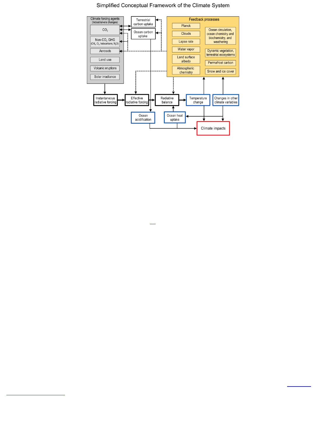
BLM 2021
Figure 8-3. Conceptualized Climate System Diagram
8.3 Past and Present Climate Impacts
According to IPCC’s climate assessment report: “Warming of the climate system is unequivocal, and since
the 1950s, many of the observed changes are unprecedented over decades to millennia. The atmosphere
and ocean have warmed, the amounts of snow and ice have diminished, sea level has risen, and the
concentration of greenhouse gases have increased.” According to IPCC’s AR5 report, the globally averaged
combined land and ocean surface temperature data, as calculated by a linear trend, show warming of 0.85 ±
0.2 °C over the period 1880 to 2012. A recent study suggests that modern global temperatures are the
highest in the last 12,000 years (Bova et al. 2021) .
Over the period 1901–2010, global mean sea level rose by 0.19 [0.17 to 0.21] meters. Rates of sea level rise
over broad regions can be several times larger or smaller than the global mean sea level rise for periods of
several decades, due to fluctuations in ocean circulation.
IPCC’s report further states that on a global scale, the ocean warming is largest near the surface, and the
upper 75 meters warmed by 0.11 [0.09 to 0.13] °C per decade over the period 1971 to 2010. Ocean warming
has dominated the increase in energy stored in the climate system, accounting for more than 90% of the
energy accumulated between 1971 and 2010. It is virtually certain that the upper ocean (0−700 m) warmed
during this period, and it likely warmed between the 1870s and 1971. There is very high confidence that the
extent of Northern Hemisphere snow cover has decreased since the mid-20th century by 1.6 [0.8 to 2.4] % per
decade for March and April, and 11.7% per decade for June, over the 1967 to 2012 period. There is high
confidence that permafrost temperatures have increased in most regions of the Northern Hemisphere since
the early 1980s, with reductions in thickness and areal extent in some regions. Based on multiple
independent analyses of measurements, it is virtually certain that globally the troposphere has warmed, and
the lower stratosphere has cooled since the mid-20th century.
The following summary text provides an overview of the highlights from the fourth iteration of the National
Climate Assessment (NCA) report. The NCA provides region-specific impact assessments for climate
change parameters that are anticipated to occur throughout this century. The global climate continues to
change rapidly compared to the pace of the natural variations in climate that have occurred throughout the
Earth’s history. Trends in globally averaged temperature, sea level rise, upper-ocean heat content, land-based
[32 ]

BLM 2021
ice melt, arctic sea ice, depth of seasonal permafrost thaw, and other climate variables provide consistent
evidence of a warming planet. These observed trends are robust and have been confirmed by multiple
independent research groups around the world (very high confidence). Many lines of evidence demonstrate
that it is extremely likely that human influence has been the dominant cause of the observed warming since
the mid-20th century. Formal detection and attribution studies for years 1951 to 2010 find that the observed
global mean surface temperature warming lies in the middle of the range of likely human contributions to
warming over that same period. Natural variability, including El Niño events and other recurring patterns of
ocean–atmosphere interactions, impact temperature and precipitation over months to years, especially at
regional scales. The global influence of natural variability, however, is limited to a small fraction of observed
climate trends over decades (very high confidence). Studies found no convincing evidence that natural
variability can account for the amount of global warming observed over the industrial era. For the period
extending over the last century, there are no convincing alternative explanations supported by the extent of
the observational evidence. Solar output changes and internal variability can only contribute marginally to
the observed changes in climate over the last century, but no convincing evidence for natural cycles in the
observational record can explain the observed changes in climate (very high confidence).
The frequency and intensity of extreme heat and heavy precipitation events are increasing in most
continental regions of the world, and these trends are consistent with expected physical responses to a
warming climate. Climate model studies are also consistent with these trends, although models tend to
underestimate the observed trends, especially for the increase in extreme precipitation events (very high
confidence for temperature, high confidence for extreme precipitation). The frequency and intensity of
extreme high temperature events are virtually certain to increase in the future as global temperature
increases (high confidence). Extreme precipitation events will very likely continue to increase in frequency
and intensity throughout most of the world (high confidence). Observed and projected trends for some other
types of extreme events, such as floods, droughts, and severe storms, have more variable regional
characteristics.
The annual average temperature over the contiguous United States has increased by 1.2ºF (0.7°C) over the
last few decades and by 1.8°F (1°C) relative to the beginning of the last century. Additional increases in
annual average temperature of about 2.5°F (1.4°C) are expected over the next few decades regardless of
future emissions, and increases ranging from 3°F to 12°F (1.6°–6.6°C) are expected by the end of century,
depending on whether the world follows a higher or lower future scenario, with proportionally greater
changes in high temperature extremes. At the regional scale, each National Climate Assessment (NCA)
region experienced increasing temperatures between 1901–1960 and 1986–2016. The largest changes were
in the western half of the United States, where average temperature increased by more than 1.5°F (0.8°C) in
Alaska, the Northwest, the Southwest, and in the Northern Great Plains. Over the entire period of record, the
Southeast has had the least warming due to a combination of natural variations and human influences; since
the early 1960s, however, the Southeast has been warming at an accelerated rate. Over the past two
decades, the number of high temperature records recorded in the United States far exceeds the number of
low temperature records. The length of the frost-free season has increased in each NCA region since the
early 1900s. The frequency of cold waves has decreased since the early 1900s, and the frequency of heat
waves has increased since the mid-1960s.
Annual average precipitation has increased by 4% since 1901 across the entire United States, with strong
regional differences: increases over the Northeast, Midwest, and Great Plains and decreases over parts of the
Southwest and Southeast consistent with the human-induced expansion of the tropics. The frequency and
intensity of heavy precipitation events across the United States have increased more than average
precipitation.

BLM 2021
8.4 BLM Fossil Fuel States Climate Change Impacts
The climate change indicators, impacts, and trends specific to states where the BLM conducts most of its
fossil fuel authorizations are subsequently described. For each state, precipitation and temperature data
from the NOAA’s climate division dataset (Vose et al. 2014) are presented to document climate trends.
Data extending back to 1895 are available for each state in the contiguous United States while the period of
record for Alaska begins in 1925. Detailed narratives for each state’s current climate conditions can be found
at NOAA with additional information provided by the Western Regional Climate Center.
Alaska
From 1925 to the mid-1970s, the statewide annual average temperature decreased by about 1°C. A major
climate shift in the Pacific Ocean during the 1976-77 winter season, detailed extensively by Miller et al.
(1994) produced many environmental impacts throughout the Pacific Basin including significant changes
in Alaskan climatology as reported by Hartmann and Wendler (2005) . Since the Pacific Ocean shift of
1976-77, the statewide annual average temperature increased by 2.5°C to 3°C with the four warmest years on
record in Alaska observed since 2014 (Figure 8-4). Most of the warming has occurred in the winter and
spring seasons, and the least amount in fall. Summer temperatures have been well above average since
1990 and winter temperatures have been above average since 2002. Some recent warming has been linked
to the Pacific Decadal Oscillation, which is a major control on Alaskan climate. However, the most recent 10-
year period (2011-2020) was over 1°C warmer than any 10-year period in the 20th century. Starting in the
1990s, high temperature records occurred three times as often as record lows, and in 2015, nine times as
frequently. However, temperature trends across the state vary considerably with the most warming observed
in the North Coast, West Coast, Central Interior, and Bristol Bay climate divisions. Since the 1970s, Arctic
and boreal regions in Alaska have experienced rapid rates of warming and thawing of permafrost.
There is no clear trend in statewide precipitation (Figure 8-4), though in the past three decades, precipitation
in the West Coast, Northeast Interior, and Central Panhandle climate divisions averaged about 10% higher
than the 1925-1999 mean. As with average precipitation, the occurrence of extreme precipitation events are
highly variable and are both regionally and seasonally dependent. Most of Alaska has seen an increase in
extreme precipitation events (the heaviest one percent of 3-day precipitation totals) since the mid-20th
century. However, there is no statewide average trend in the number of days with precipitation exceeding 1
inch since 1950, and the highest values occurred in the 1930s.
Late summer Arctic sea ice extent and thickness has decreased substantially in the last several decades, and
the ice volume is approximately half of that observed prior to satellite monitoring in 1979. Since the early
1980s, annual average arctic sea ice extent has decreased between 3.5% and 4.1% per decade, and
September sea ice extent, which is the annual minimum extent, has decreased between 10.7% and 15.9% per
decade. The lowest minimum Arctic sea ice extent occurred in 2012. Arctic sea ice plays a vital role in the
climate of Alaska, the lives of its inhabitants, and the functionality of its ecosystems. Warming linked to ice
loss influences atmospheric circulation and precipitation patterns, both within and beyond the Arctic. With
the late-summer ice edge located farther north than it used to be, storms produce larger waves and cause
more coastal erosion. A significant increase in the number of coastal erosion events has been observed as
the protective sea ice embankment is no longer present during the fall months. In response to the increased
erosion, several coastal communities are seeking to relocate.
Glaciers continue to melt in Alaska, with an estimated loss of 75 ± 11 gigatons (Gt) of ice volume per year
from 1994 to 2013, 70% of which is coming from land-terminating glaciers; this rate is nearly double the
[33 ]
[34 ]
[35 ]
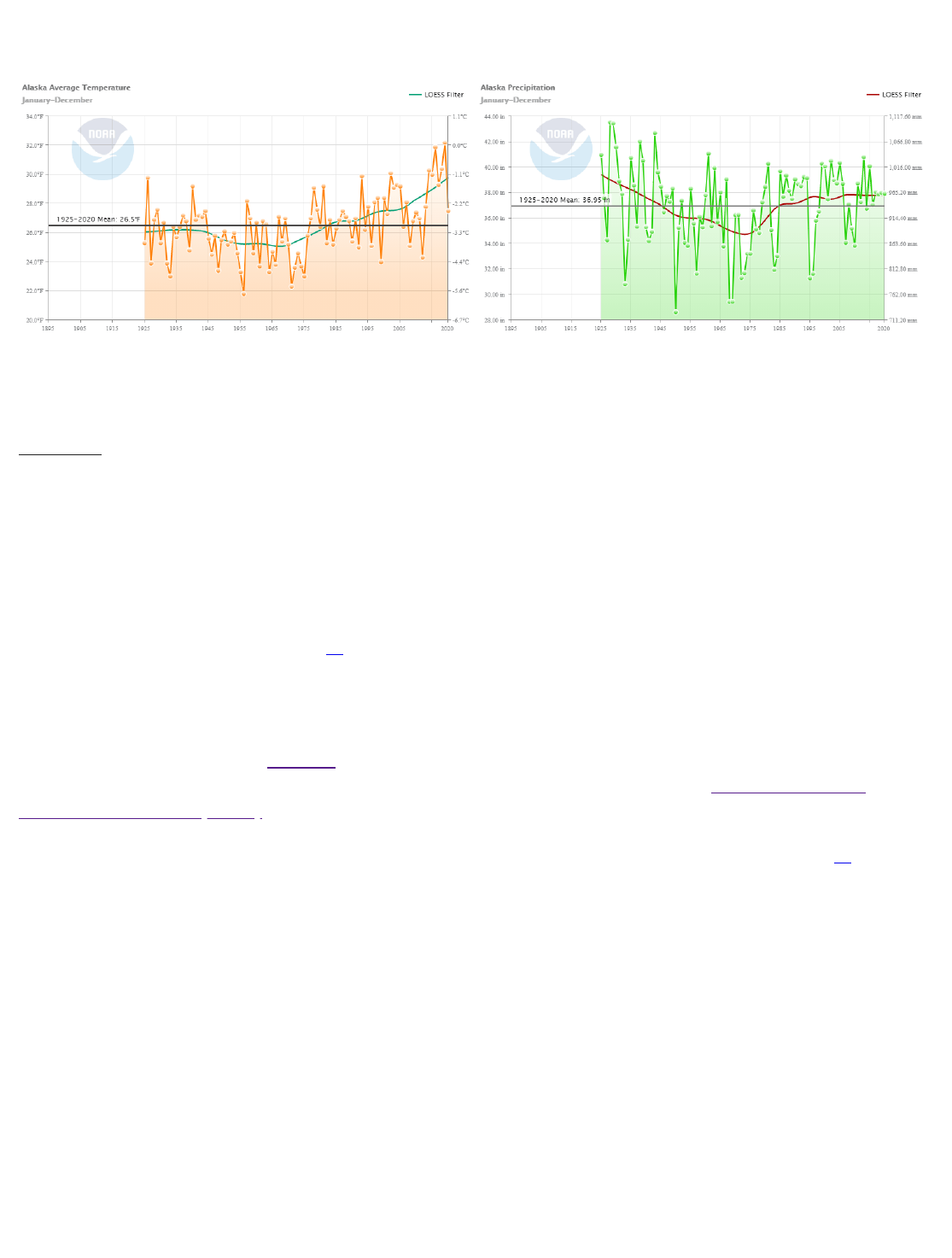
BLM 2021
1962–2006 rate. Melting glaciers are likely to produce uncertainties for hydrologic power generation, which
is an important resource in Alaska.
(a) (b)
Figure 8-4. AK Temperature and Precipitation Records
California
The average annual temperatures in California have increased by nearly 3°F since the beginning of the 20th
century (Figure 8-5). The years 2014 and 2015 were the first and second warmest, respectively, in the 126-
year record, and the most recent 10-year period (2011-2020) was the warmest on record. Since 1995,
California has experienced a below normal number of cold nights and its highest number of very warm nights
over the historical record. The record warmth in 2014 and 2015, in combination with multiple years of below
average precipitation including the driest year (Figure 8-5) led to the most severe drought of the past 1,200
years (Griffin and Anchukaitis 2014) .
While there is no long-term trend in statewide precipitation (Figure 8-5), 2013 and 2020 were the driest and
third driest years, respectively, in the 126-year record. Like precipitation, the state’s snowpack varies greatly
from year to year. During the SNOTEL monitoring era, which begins around 1980, snowpack has decreased
slightly in the state’s major river basins. According to data provided by the USDA’s Natural Resources
Conservation Service (NRCS), statewide April 1 snowpack has averaged about 10% lower during the first two
decades of the 21st century as compared to the last two decades of the 20th century, with 2015 likely
featuring the lowest snowpack in the Sierra Nevada in the last 500 years (Belmecheri et al. 2015) .
Many coastal resources in the state have been affected by sea level rise, ocean warming, reduced ocean
oxygen, and ocean acidification—all impacts of human-caused climate change. At the Golden Gate Bridge in
San Francisco, sea level rose 9 inches (22 cm) between 1854 and 2016, and in San Diego, sea level rose 9.5
inches (24 cm) from 1906 to 2016.
[36 ]
[37 ]
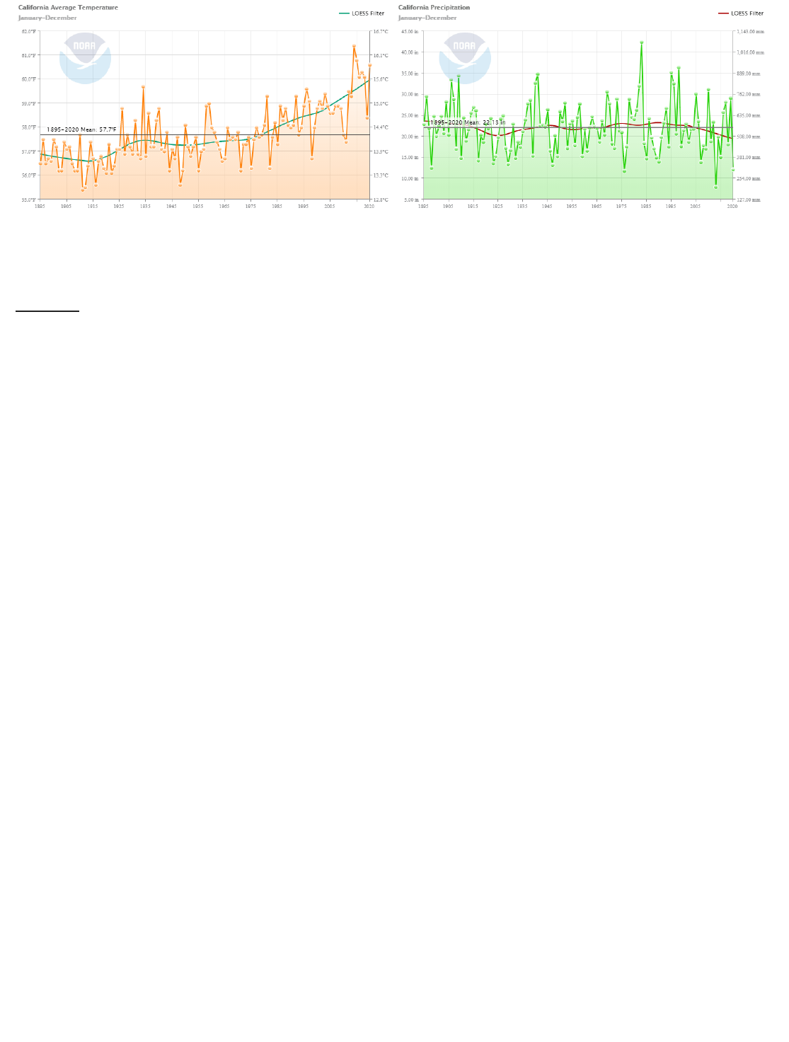
BLM 2021
(a) (b)
Figure 8-5. CA Temperature and Precipitation Records
Colorado
Since the start of the 20th century, the average annual temperature in Colorado increased by approximately
2.5°F (Figure 8-6). Six of the eight hottest years in the state’s recorded history have occurred since 2012, and
the most recent 10-year period (2011-2020) was the hottest yet observed. While temperatures have
increased statewide, the Colorado Basin (Colorado Climate Division 2) has warmed by nearly twice as much
as either the Arkansas Basin (Colorado Climate Division 1) or the Rio Grande Basin (Colorado Climate
Division 5). In addition to the overall trend of higher average temperatures, the state has experienced an
above average number of very hot days (days with a maximum temperature exceeding 95°F) and a decrease
in the number of very cold nights (days with a minimum temperature below 0°F) since 1990. Warming has
occurred in all seasons and has been observed throughout the state. Daily minimum temperatures increased
more than daily maximum temperatures. Increased temperatures have contributed to earlier snowmelt and
peak runoff timing during spring by 1 to 4 weeks. The growing season (i.e., frost-free days) has increased by
nearly 3 weeks since 1991 relative to the 1901 to 1960 average.
Long-term average annual precipitation has been variable, though Colorado has generally experienced above
average fall precipitation since 1980 and below average spring precipitation since 2000. Unlike many areas
of the United States, Colorado has not experienced an upward trend in the frequency of extreme precipitation
events. Drought reconstructions from tree rings indicate that droughts are a frequent occurrence in
Colorado, and episodes more severe than any in the historical record have occurred in the more distant past.
Despite historically low snowpack in 2012, there is no long-term trend in April 1 snowpack water at Berthoud
Pass, which has one of the state’s longer snow course sampling histories. However, there is considerable
site-specific variability among Colorado snow course locations, with some indicating no long-term trend
while others show a significant decrease in April 1 snowpack. Snowpack data from the NRCS show that
during the most recent 40 years covered by SNOTEL data, year-to-year variability in basin-specific and
statewide April 1 snowpack is large, though in general, snowpack has been slightly lower in the most recent
20-year period.
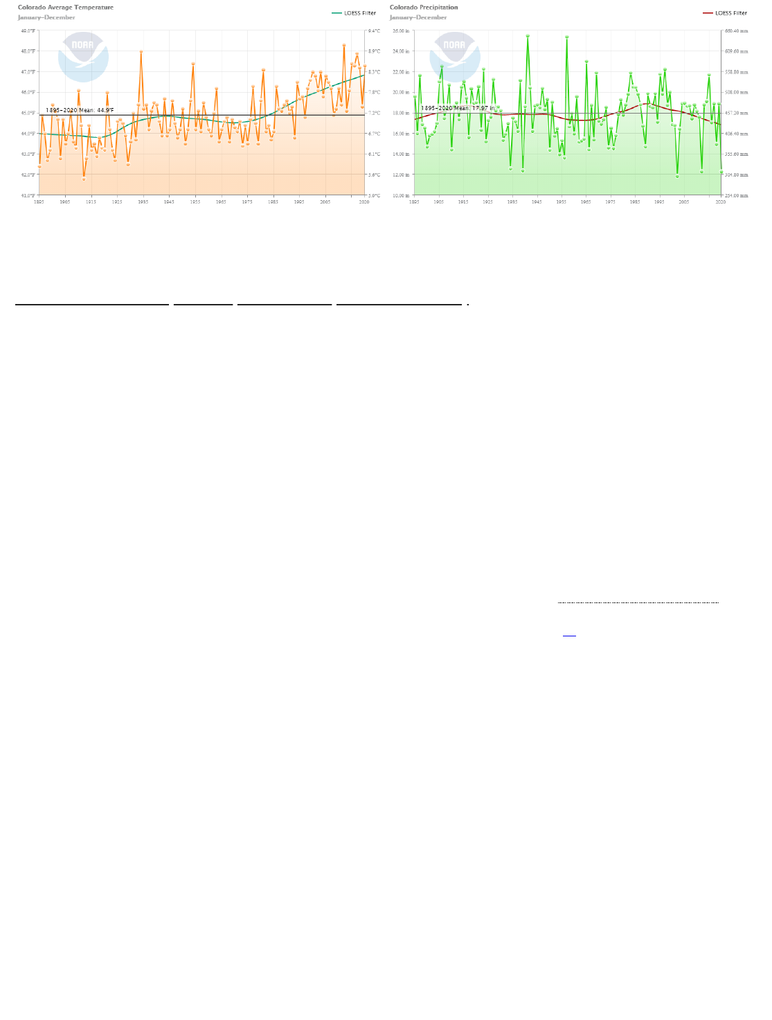
BLM 2021
(a) (b)
Figure 8-6. CO Temperature and Precipitation Records
Northern Great Plains (Montana, North Dakota, and South Dakota)
Since the start of the 20th century, Montana and the Dakotas have warmed by about 2.5°F. Since 1981, 8 and
9 of the hottest years on record have occurred in the Dakotas and Montana, respectively. While temperatures
have increased in all seasons, the largest increase has occurred in winter and spring. For example, over the
past 130 years, winter temperatures in North Dakota have increased by 4.4°F per century, more than three
times as much as the summer trend of 1.4°F per century. Warmer temperatures have extended the growing
season by as much as 30 days in the northern Great Plains.
There is no clear long-term trend in Montana precipitation, but in the Dakotas, annual precipitation amounts
have increased, and rainstorms are becoming more intense. Over the last 50 years in the Great Plains, the
amount of rain falling during the wettest 4 days of the year increased by approximately 15%. Increasing
rainfall could benefit some farms but also may increase the risk of flooding.
Despite warming temperatures, NRCS snowpack data show that average April 1 in
Montana has not changed during the SNOTEL era. However, since 1955, longer term snow course data
indicate a significant decrease in Montana’s April 1 snowpack (Mote et al. 2018) .
Rising temperatures and recent droughts have killed many trees by drying out soils, increasing the risk of
forest fires, or enabling outbreaks of forest insects. In the coming decades, the changing climate is likely to
decrease the availability of water in Montana, affect agricultural yields, and further increase the risk of
wildfires.
snow-water equivalents
[38 ]
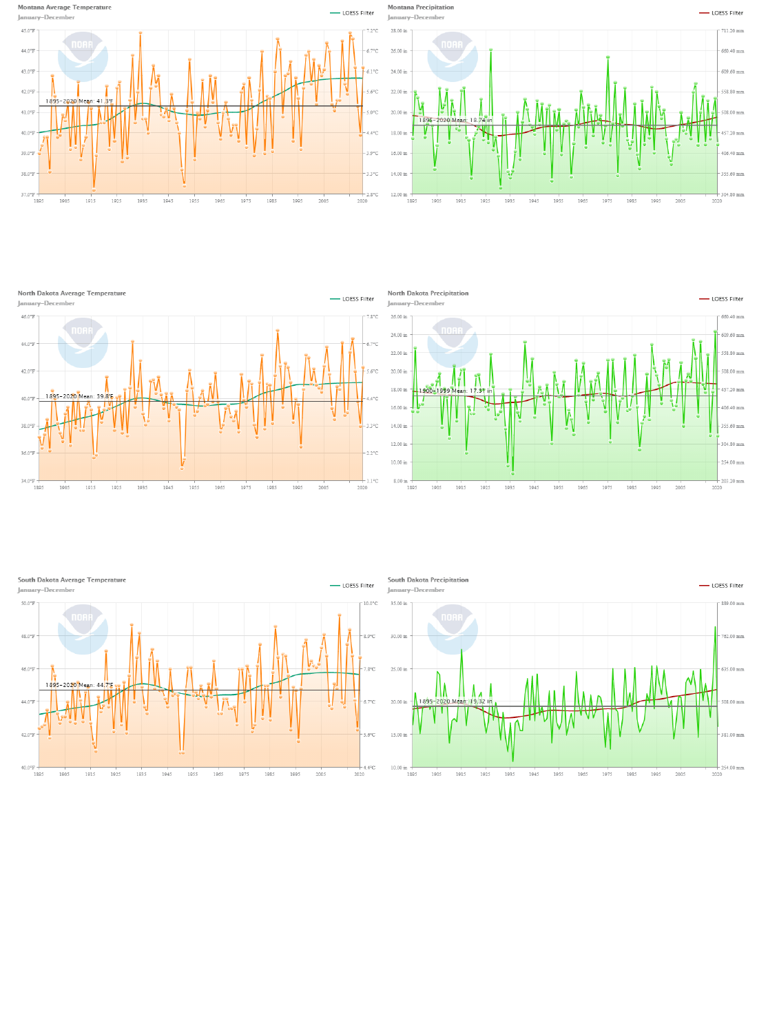
BLM 2021
(a) (b)
Figure 8-7. MT Temperature and Precipitation Records
(a) (b)
Figure 8-8. ND Temperature and Precipitation Records
(a) (b)
Figure 8-9. SD Temperature and Precipitation Records
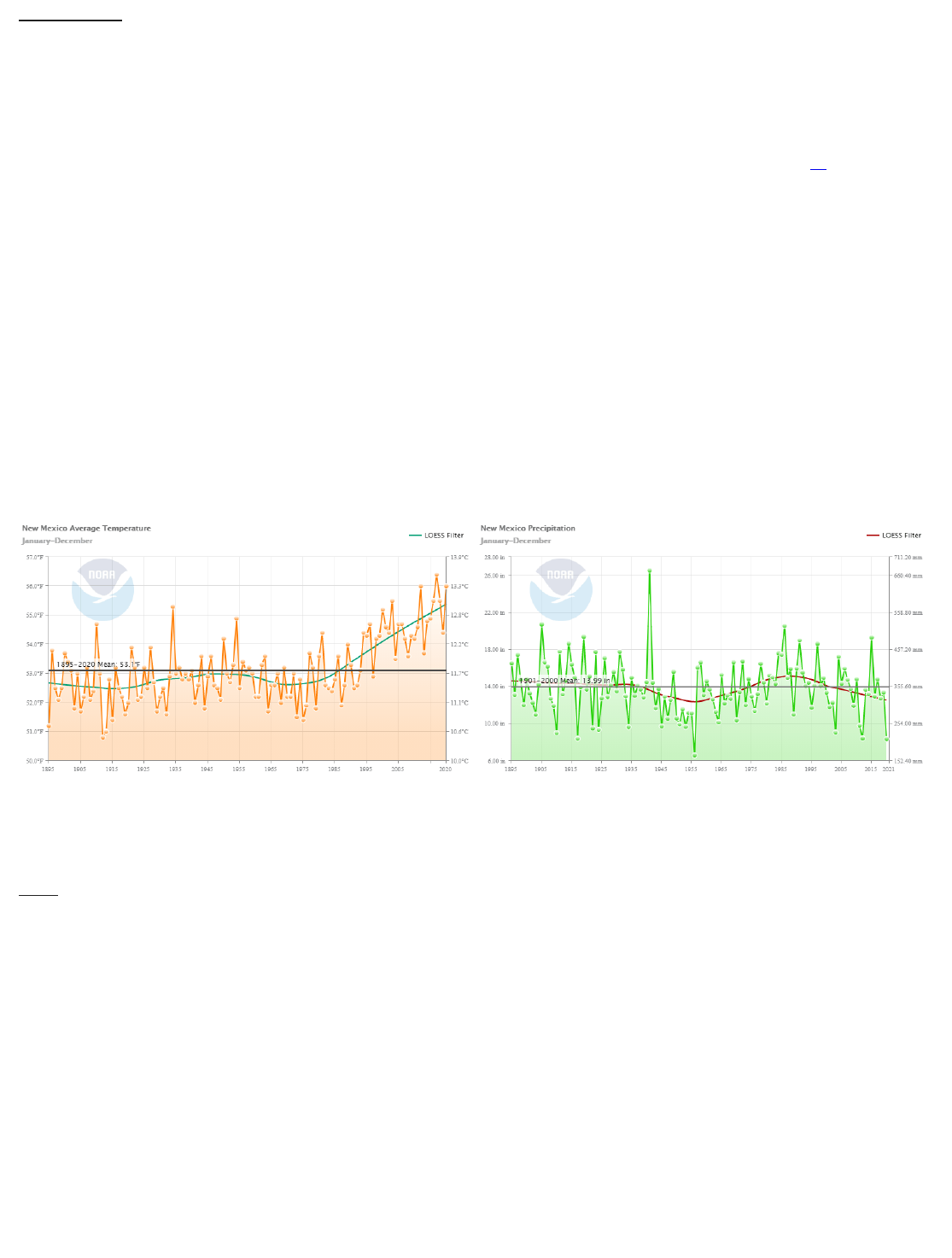
BLM 2021
New Mexico
From 1895 to the end of the 1970s, there was no trend in New Mexico mean annual temperature, but since
1980, the mean annual temperature increased by approximately 2.5°F (Figure 8-10). The last decade (2011-
2020) was the warmest on record for the state, and the 3 hottest years observed each occurred since 2012.
Temperatures have increased the most in the central and southeastern portions of the state while the
northeastern plains and Mogollon Rim have warmed by about half as much (Vose et al. 2017 ) . Along
with higher mean temperatures, much of the state has seen increases in the number of extremely hot days
(maximum temperature at or above 100°F), especially on the eastern plains.
There is large interannual and interdecadal variability in New Mexico precipitation (Figure 8-10). While 2020
was the second driest year on record and the most recent decade (2011-2020) was the driest since 1955-
1964, there is no long-term trend in mean annual precipitation. Statewide annual precipitation has ranged
from a high of 26.57 inches in 1941 to a low of 6.58 inches in 1956. Unlike many areas of the United States,
there has been no increase in the frequency of extreme precipitation events (days with an inch or more of
precipitation) in New Mexico. While the average number of such events between 2015 and 2018 period was
the highest on record, it is too short a period to constitute a trend. Drought reconstructions from tree rings
indicate that droughts are a frequent occurrence in New Mexico, and episodes more severe than any in the
recent historical record have occurred in the more distant past.
(a) (b)
Figure 8-10. NM Temperature and Precipitation Records
Utah
The early 21st century has been the warmest period on record for Utah (Figure 8-11). Since 1895,
temperatures have been increasing 0.2ºF to 0.3 ºF per decade in each of Utah’s seven climate divisions. The
period from 2000 to 2004 had the largest number of extremely hot days with maximum temperature at or
above 100°F in the historical record. In addition to the overall trend of higher temperatures, the state has
experienced a marked increase in the number of very warm nights (minimum temperature at or above 75°F)
and a decrease in the number of very cold nights (minimum temperature at or below 0°F) since 1990. While
2020 was the driest year on record for Utah and 21st century precipitation has averaged a few percent below
the long-term mean across Utah, there is no statistically significant trend in precipitation for the state or in
any climate division with natural variability resulting in both wetter and drier periods than observed in the
past two decades (Figure 8-11). As the state has warmed, the percentage of precipitation falling as snow
during the winter has decreased, as has snow depth and snow cover.
[39 ]
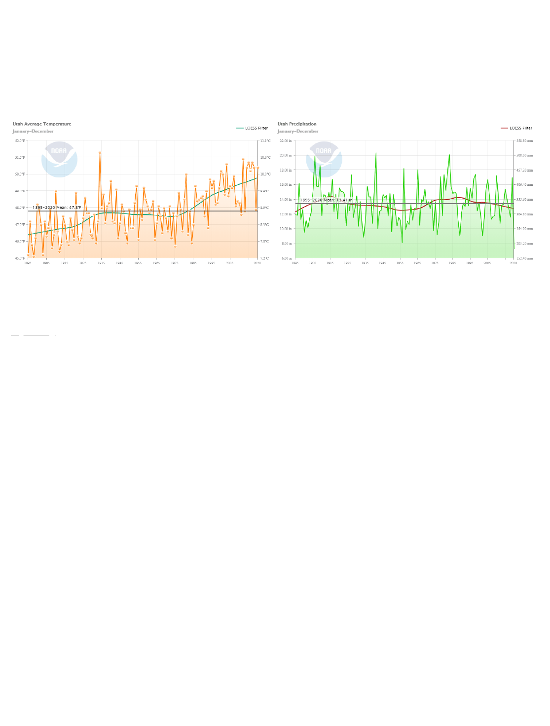
BLM 2021
April 1 snowpack across the state has gradually decreased in the past 40 years with 2011-2020 average
statewide snowpack approximately 20% lower than that observed between 1981-1990. Utah frequently
experiences droughts. Since snowmelt from the snowpack provides water for many river basins, abnormally
low winter and spring precipitation is often the trigger for drought conditions. In 2012, Utah experienced one
of its driest springs since records began in 1895, resulting in severe drought conditions in areas across the
entire state. The historical record indicates periodic occurrences of extended wet and dry periods. Dry
conditions since 2000 have resulted in near-record-low water levels in the Great Salt Lake.
(a) (b)
Figure 8-11. UT Temperature and Precipitation Records
Wyoming
The 21st century has been the warmest period on record for Wyoming, with a net warming of 1.4°F since the
beginning of the 20th century (Figure 8-12). Three of the four hottest years on record have occurred since
2012, with that year the hottest in the 126-year observational period. Temperature increases have been
observed in all seasons. Since 1995, winter and summer temperatures have averaged 1.9°F and 1.2°F above
the historical average, respectively. The state has experienced an above average frequency of very hot days
(days with maximum temperature above 95°F) since 2000. Wyoming rarely experiences warm nights (days
with minimum temperatures above 70°F), but the early part of the 21st century has seen an above average
number of such nights. In addition to the overall trend of higher average temperatures, the state has
experienced a below average number of very cold days (days with maximum temperatures below 0°F) since
2000.
There is no long-term trend in statewide annual mean precipitation (Figure 8-12), though 2012 was the driest
year on record and 2020 the fifth driest on record. The driest multiyear periods were in the 1930s, 1950s,
and 2000s, and the wettest in the 1940s and 1990s. The driest 5-year period was 1931–1935 and the
wettest was 1995–1999. Unlike many other areas of the western United States, April 1 snowpack has
remained relatively constant over the past 40 years. The median statewide April 1 snowpack between 1981-
2000 is the same as that observed during the most recent 10-year period (2011-2020).

BLM 2021
(a) (b)
Figure 8-12. WY Temperature and Precipitation Records
* * *

BLM 2021
9.1 Representative Concentration Pathways
The current understanding of the climate system comes from the cumulative results of observations,
experimental research, theoretical studies, and model simulations conducted by thousands of scientists from
all over the world. Climate change is fundamentally a cumulative phenomenon, global in scope, and all GHGs
contribute incrementally to climate change regardless of scale or origin. The multitude of interwoven natural
systems and feedback mechanisms that contribute to climate variability over the entirety of Earth further
complicate analysis.
Climate scientists provide analysis by modeling changes to these systems in response to a range of global
emissions scenarios known as Representative Concentration Pathways (RCPs). The RCPs are not fully
integrated scenarios of climate feedback, policy, emissions limits, thresholds, or socioeconomic projections,
but rather a consistent set of cumulative emissions projections out to year 2100 of only the components of
radiative forcing that are meant to serve as input for climate and atmospheric chemistry modeling. There are
four scenarios that climate scientists have used for assessment in the Coupled Model Intercomparison
Project Phase 5 (CMIP5) (Figure 9-1).
RCP2.6
- A low emissions pathway that is representative of scenarios that lead to very low atmospheric
GHG concentrations. Radiative forcing levels reach a peak around 3.1 W/m by mid-century, returning
to 2.6 W/m by 2100. To reach these radiative forcing levels, global GHG emissions are reduced
substantially over time. This scenario also assumes there will be “negative emissions” starting in 2080,
with more carbon being removed from the atmosphere than is emitted. The aggregate global emissions
of this pathway is approximately 1,715.7 GtCO2e (2018 - 2100). CO alone represents 54.2% of the total
contributing emissions, and 81.5% of the total CO emissions are attributable to fossil fuel use.
RCP4.5
- Stabilization scenario where total radiative forcing stabilizes at 4.5 W/m before 2100 by
employment of a range of technologies and strategies for reducing GHG emissions. This pathway
forecasts global emissions increasing until about 2040, and then declining starting in 2050. The
aggregate emissions of this pathway is approximately 3,728.6 GtCO2e (2018 - 2100). CO alone
represents 67% of the total contributing emissions, and 98.2% of the total CO emissions are
attributable to fossil fuel use.
RCP6.0
Stabilization scenario where total radiative forcing stabilizes at of 6.0 W/m after 2100 by
employment of a range of technologies and strategies for reducing GHG emissions. Emissions of CO
grow steadily until 2080 before declining. The cumulative emissions of this pathway are approximately
5,380.2 GtCO e (2018 - 2100). CO alone represents 74.3% of the total contributing emissions and,
101.1% of the total CO emissions are attributable to fossil fuel use. Please note, the Land Use Change
(LUC) CO emissions in this scenario are negative at about the mid-century mark, which produces data
showing fossil fuel emissions that are greater than the total emissions (which include the negative LUC
values).
RCP8.5
- Pathway scenario with increasing emissions over time that leads to very high GHG
concentration levels and radiative forcing of 8.5 W/m in 2100. This pathway assumes emissions
trajectories follow historical growth and assumes no climate policies are enacted to reduce emissions.
2
2
2
2
2
2
2
2
2
2 2
2
2
2
9.0 Projected Climate Change
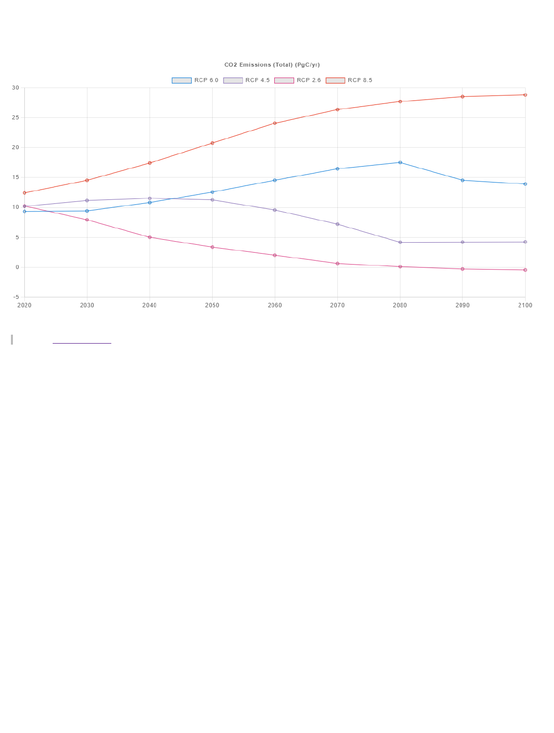
BLM 2021
The aggregate emissions of this pathway are approximately 9,227.7 GtCO2e (2018 - 2100). CO alone
represents 72.3% of the total contributing emissions, and 97.8% of the total CO emissions are
attributable to fossil fuel use.
Figure 9-1. RCP Data Time Series - CO2 Emissions
Source: RCP Database
The future climate equilibrium is dependent upon warming caused by past anthropogenic emissions, future
anthropogenic emissions, and natural variability. Global mean surface temperature change for the period
2016–2035 relative to 1986–2005 is similar for the four modeled RCPs and will likely be in the range of 0.3°C
to 0.7°C (medium confidence). The projection assumes no major volcanic eruptions, changes in natural
emissions sources (e.g., CH and N O), or unexpected changes in total solar irradiance. By 2050, the
magnitude of the projected climate change is substantially affected by the overall emissions path along
which the world is tracking. It should be noted that according to the IPCC, only emissions projections
following the lowest concentration pathway (RCP2.6) result in an estimated mean increase in global average
temperatures below 2°C. Equally important, IPCC scientists project warming will continue beyond 2100
under all RCP scenarios except for RCP2.6.
The projected increase of global mean surface temperature by the end of the 21st century (2081–2100)
relative to 1986–2005 is likely to be 0.3°C to 1.7°C under RCP2.6, 1.1°C to 2.6°C under RCP4.5, 1.4°C to 3.1°C
under RCP6.0, and 2.6°C to 4.8°C under RCP8.5. As global mean surface temperature increases, it is virtually
certain that there will be more frequent hot and fewer cold temperature extremes over most land areas on
daily and seasonal timescales. It is also very likely that heat waves will occur with a higher frequency and
longer duration. Occasional cold winter extremes will continue to occur due to the inherent variability within
the climate system. Changes in precipitation patterns will not be uniform, but in general, scientists expect
arid regions to become drier and wetter areas to experience frequent exceptional precipitation events.
Oceans will continue to warm, with the greatest impacts occurring at the surface of tropical and northern
hemisphere subtropical regions. Models also predict ocean acidification will increase for all RCP scenarios,
where surface pH can be expected to decrease by 0.06 to 0.07 (15 to 17%) for RCP2.6 and 0.14 to 0.15 (38 to
41%) for RCP4.5. Year-round reductions in Arctic sea ice are projected for all RCP scenarios, and it is
virtually certain that near-surface (upper 3.5 m) permafrost extent at high northern latitudes will be reduced
2
2
4 2

BLM 2021
(37% - RCP2.6 to 81% - RCP8.5) as the global mean surface temperature increases. Global mean sea level
rise will very likely continue at a faster rate than observed from 1971 to 2010. For the period 2081–2100
relative to 1986–2005, the rise will likely be in the range of 0.26 to 0.55 m for RCP2.6 and of 0.45 to 0.82 m
for RCP8.5. It is very likely that the sea level will rise in more than 95% of the ocean area, where about 70%
of coastlines worldwide would experience a sea level change within ±20% of the global mean.
9.2 Shared Socioeconomic Pathways
In preparation for the IPCC's Sixth Assessment Report (AR6), the climate science research community,
economists, and energy systems modelers developed a new range of “pathways” that examine how global
society, demographics, and economics might influence future climate impacts, vulnerabilities, adaptation,
and mitigation over the next century. The scenarios are collectively known as the Shared Socioeconomic
Pathways (SSPs). These new scenarios are being used to inform the next round of climate modeling that is
being incorporated into AR6. The RCPs and SSPs are meant to complement each other. The RCPs set
pathways for GHG concentrations and the potential amount of radiative forcing and warming the world may
experience by the end of the century. The SSPs explore how reductions in emissions will, or will not, be
achieved and can therefore be thought of as potential mitigation alternatives.
There are five basic SSP narratives that were developed. The SSP scenarios provide a range of plausible
trends (Figure 9-2) that could shape future society and include the following:
SSP1 (Low challenges to mitigation and adaptation)
– The world shifts gradually, but pervasively,
toward a more sustainable path, emphasizing more inclusive development that respects perceived
environmental boundaries. Management of the global commons slowly improves, educational and
health investments accelerate the demographic transition, and the emphasis on economic growth shifts
toward a broader emphasis on human well-being. Driven by an increasing commitment to achieving
development goals, inequality is reduced both across and within countries. Consumption is oriented
toward low material growth and lower resource and energy intensity.
SSP2 (Medium challenges to mitigation and adaptation)
- The world follows a path in which social,
economic, and technological trends do not shift markedly from historical patterns. Development and
income growth proceeds unevenly, with some countries making relatively good progress and others
falling short of expectations. Global and national institutions work toward but make slow progress in
achieving sustainable development goals. Environmental systems experience degradation, although
there are some improvements, and overall the intensity of resource and energy use declines. Global
population growth is moderate and levels off in the second half of the century. Income inequality
persists or improves only slowly, and challenges to reducing vulnerability to societal and environmental
changes remain.
SSP3 (High challenges to mitigation and adaptation)
- A resurgent nationalism, concerns about
competitiveness and security, and regional conflicts push countries to increasingly focus on domestic
or, at most, regional issues. Policies shift over time to become increasingly oriented toward national
and regional security issues. Countries focus on achieving energy and food security goals within their
own regions at the expense of broader-based development. Investments in education and technological
development decline. Economic development is slow, consumption is material-intensive, and
inequalities persist or worsen over time. Population growth is low in industrialized and high in
developing countries. A low international priority for addressing environmental concerns leads to
strong environmental degradation in some regions.
[40 ]

BLM 2021
SSP4 (Low challenges to mitigation, high challenges to adaptation)
- Highly unequal investments in
human capital, combined with increasing disparities in economic opportunity and political power, lead
to increasing inequalities and stratification both across and within countries. Over time, a gap widens
between an internationally-connected society that contributes to knowledge- and capital-intensive
sectors of the global economy, and a fragmented collection of lower-income, poorly educated societies
that work in a labor intensive, low-tech economy. Social cohesion degrades and conflict and unrest
become increasingly common. Technology development is high in the high-tech economy and sectors.
The globally connected energy sector diversifies, with investments in both carbon-intensive fuels like
coal and unconventional oil, but also low-carbon energy sources. Environmental policies focus on local
issues around middle and high income areas.
SSP5 (High challenges to mitigation, low challenges to adaptation)
- This world places increasing faith
in competitive markets, innovation, and participatory societies to produce rapid technological progress
and development of human capital as the path to institutions to enhance human and social capital. At
the same time, the push for economic and social development is coupled with the exploitation of
abundant fossil fuel resources and the adoption of resource and energy intensive lifestyles around the
world. All these factors lead to rapid growth of the global economy, while global population peaks and
declines in the 21st century. Local environmental problems like air pollution are successfully managed.
There is faith in the ability to effectively manage social and ecological systems, including by geo-
engineering if necessary.
Both SSP1 and SSP5 consider optimistic scenarios for human development with substantial investments in
education, rapid economic growth, and technology. They differ in that SSP5 assumes that development is
driven by fossil fuel energy, while in SSP1 there is a shift towards sustainable practices and sustainable
development. Global markets are increasingly integrated. There are also strong investments in health,
education, and renewable energy sources. The SSP2 scenario represents a “middle of the road” path that
follows historical development trends throughout the 21st century. While SSP3 and SSP4 present less
optimistic economic and social development scenarios, with little investment in education or health in poorer
countries coupled with a fast-growing population and increasing inequalities. Each SSP has a baseline
scenario that describes future developments in the absence of new climate policies, beyond those already in
place today. The SSPs can then be combined with various emission mitigation objectives to identify how
each of the different RCPs can be achieved.
To understand how the SSPs relate to different levels of warming under the RCP scenarios, six different
integrated assessment models (IAMs) were used. The IAMs produce an estimate of the GHG emissions that
would occur based on socioeconomic factors outlined in the SSPs. The resulting emissions were then used
as inputs for the Model for the Assessment of Greenhouse Gas Induced Climate Change (MAGICC) to provide
estimates of atmospheric GHG concentrations and future warming. In addition to the four RCP’s analyzed in
AR5, three additional RCPs representing radiative forcing of 1.9, 3.4, and 7.0 W/m were evaluated to expand
the range of emissions mitigation targets. The RCP1.9 represents a pathway that limits warming to 1.5°C.
The combination of five SSPs and six of the RCPs is shown in Figure 9-1 (a). Each box in the slide shows the
number of models that were able to successfully reach the RCP target, out of the total number of models
available for a given SSP. For example, the “3/4” in the SSP5 / RCP2.6 cell means that four IAMs tried to
achieve RCP2.6 in an SSP5 world, but only three of the models could find a solution. The other model could
not either reduce emissions fast enough or generate sufficient negative emissions. Similarly, only SSP5
could generate scenarios that reached RCP8.5 levels of radiative forcing, while emissions were too low in
other SSP baselines. This research shows that some mitigation and adaptation to climate change is much
easier under some SSP scenarios than others and not all SSPs are compatible with RCPs that limit warming
to 1.5°C or 2°C above pre-industrial levels. However, even though not all the IAMs find a viable solution for
2
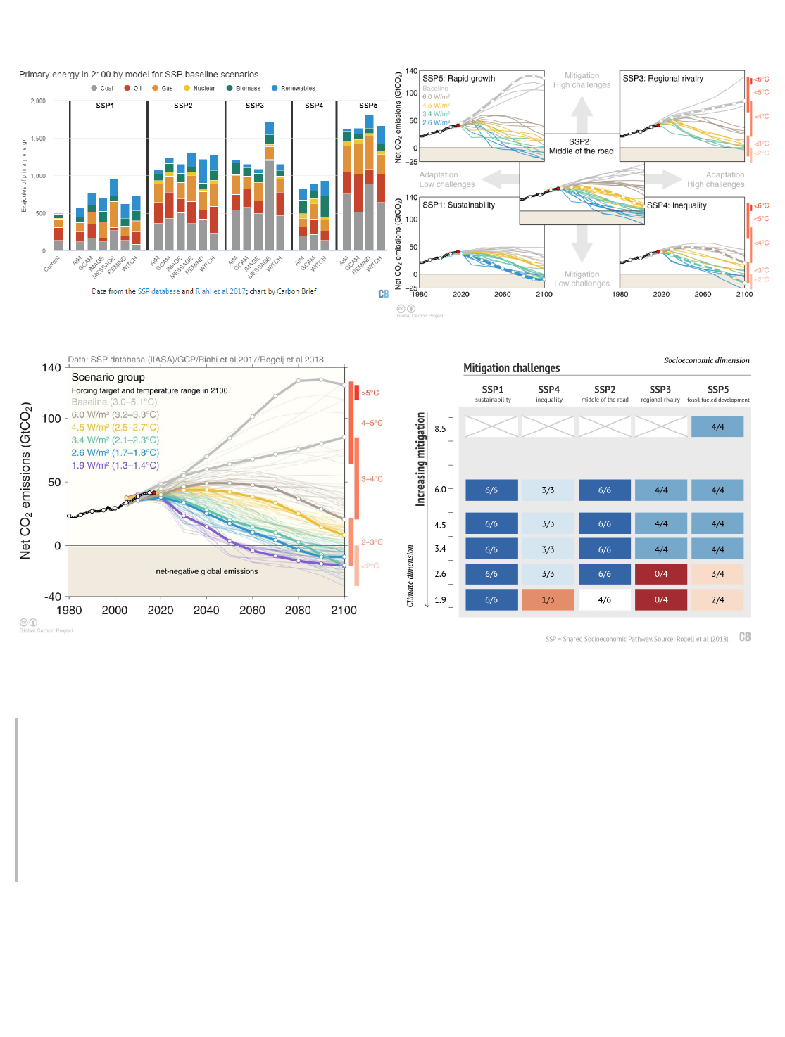
BLM 2021
scenarios that limit warming below 1.5°C or 2°C, it does not necessarily mean that these scenarios are
impossible. Models are imperfect and cannot foresee all changes that will happen over the next century.
(a) (b)
(c) (d)
Figure 9-2. Shared Socioeconomic Pathways
(a) - Global primary energy use by fuel type in 2100 in exajoules (EJ) for baseline scenarios in each IAM and SSP. Current
energy use (as of 2010) is shown for reference in the far left bar. Data from the SSP database and Riahi et al 2017;
(b) - Global CO2 emissions (GtCO2) for all IAM runs in the SSP database separated out by SSP. Chart via Glen Peters and
Robbie Andrews and the Global Carbon Project.
(c) - Global CO2 emissions (gigatonnes, GtCO2) for all IAM runs in the SSP database. SSP no-climate-policy baseline
scenarios are shown grey, while various mitigation targets are shown in color. Bold lines indicate the subset of scenarios
chosen as a focus for running CMIP6 climate model simulations. Chart produced for Carbon Brief by Glen Peters and
Robbie Andrews from the Global Carbon Project.
(d) - Combination of SSP and RCP model runs in the SSP database, with RCPs listed in order of increasing mitigation and
SSPs in the (rough) order of increasing mitigation difficulty. Ratios in cells indicate the number of models that
succeeded in making the scenario “work” out of the total number of models available for the SSP. Chart by Carbon Brief,
adapted from Figure S1 in Rogelj et al (2018).

BLM 2021
9.3 Special Report 1.5
In 2018, the IPCC released its "Special Report: Global Warming of 1.5°C" which describes the predicted
impacts of global warming of 1.5°C above pre-industrial temperature levels and the related global
greenhouse emission pathways to limit warming below 2°C. The report presents its conclusions based on
the assessment of the available scientific, technical, and socioeconomic information related to global
warming of 1.5°C and 2.0°C. Key findings are excerpted here.
Human activities are estimated to have caused approximately 1.0°C of global warming above pre-
industrial levels, with a likely range of 0.8°C to 1.2°C, and warming is likely to reach 1.5°C between 2030
and 2052 if it continues to increase at the current rate. Warming from anthropogenic emissions from
the pre-industrial period to the present will persist for centuries to millennia and will continue to cause
further long-term changes in the climate system, but these emissions alone are unlikely to cause global
warming of 1.5°C (medium confidence).
Climate models project robust differences in regional climate characteristics between the present
observed shifts and global warming of 1.5°C, and warming between 1.5° C and 2°C. These differences
include increases in: mean temperature in most land and ocean regions (high confidence), hot extremes
in most inhabited regions (high confidence), heavy precipitation in several regions (medium confidence),
and the probability of drought and precipitation deficits in some regions (medium confidence).
By 2100, global mean sea level rise is projected to be around 0.1 meters lower with global warming of
1.5°C compared to 2°C (medium confidence). Sea level will continue to rise well beyond 2100 (high
confidence), and the magnitude and rate of this rise depend on future emission pathways. A slower
rate of sea level rise enables greater opportunities for adaptation in the human and ecological systems
of small islands, low-lying coastal areas, and deltas (medium confidence).
Limiting global warming to 1.5°C compared to 2°C is projected to reduce increases in ocean
temperature as well as associated increases in ocean acidity and decreases in ocean oxygen levels
(high confidence), all of which will reduce risks to marine biodiversity, fisheries, and ecosystems, and
their functions and services to humans.
9.4 State Climate Change Projections
The following climate change discussion summarizes information from NCA4 and NOAA’s state climate
summaries (including all data in Figure 9-3).
Alaska
Alaska is on the front lines of climate change and is among the fastest warming regions on Earth. It is
warming faster than any other state, and it faces a myriad of issues associated with a changing climate.
Global climate models project more warming in the Arctic and interior areas than in the southern areas of
Alaska. In the RCP8.5 scenario, interior and northern areas of the state are projected to warm by 10°–16°F,
southern portions by 2.5°–8°F. Climate models suggest that Arctic waters will be virtually ice-free by late
summer before 2050 and near-surface permafrost will likely disappear on 16% to 24% of the landscape by
the end of the 21st century.
Average precipitation is projected to increase in all seasons during the 21st century, with the greatest
increases expected in winter and spring. By the middle of the 21st century, annual precipitation increases
[41 ]

BLM 2021
are projected to exceed 10% over most of the state, with greater increases in the Arctic and interior and the
largest increases in the northeastern interior.
Climatic extremes are expected to change with the changing climate. Under a higher scenario (RCP8.5), by
mid-century (2046–2065) the highest daily maximum temperature (the hottest temperature one might expect
on a given summer day) is projected to increase 4°–8°F compared to the average for 1981–2000. For the
same future period (2046–2065), the lowest daily maximum temperature (the highest temperature of the
coldest day of the year) throughout most of the state is projected to increase by more than 10°F, with smaller
projected changes in the Aleutian Islands and southeastern Alaska. Additionally, the lowest daily minimum
temperatures (the coldest nights of the year) are projected to increase by more than 12°F. The number of
nights below freezing would likely decrease by at least 20 nights per year statewide, and by greater than 45
nights annually in coastal areas of the North Slope, Seward Peninsula, Yukon–Kuskokwim Delta, Alaska
Peninsula, and Southcentral Alaska. Annual maximum one-day precipitation is projected to increase by 5%–
10% in southeastern Alaska and by more than 15% in the rest of the state, although the longest dry and wet
spells are not expected to change over most of the state. Growing season length (the time between last and
first frosts in a given year) is expected to increase by at least 20 days and perhaps more than 40 days
compared to the 1982–2010 average. Whether or not this increased growing potential is realized will largely
depend on soil conditions and precipitation.
The area burned by wildfires may increase further under a warming climate. Projections of burned area for
2006–2100 are 98 million acres under a lower scenario (RCP4.5) and 120 million acres under a higher
scenario (RCP8.5).
California
Under a higher emissions pathway, historically unprecedented warming is projected by the end of the 21st
century. Even under a pathway of lower GHG emissions, average annual temperatures are projected to most
likely exceed historical record levels by the middle of the 21st century. However, there is a large range of
temperature increases under both pathways, and under the lower pathway a few projections are only slightly
warmer than historical records. Overall, any warming will lead to increased heat wave intensity but
decreased cold wave intensity. Future heat waves could particularly stress coastal communities, such as
San Francisco, that are rarely exposed to extreme temperatures and therefore are not well adapted to such
events. More intense, longer-lasting heat waves will result in increasing peak demands for electricity for air
conditioning, depleting electrical generation and distribution capacities, resulting in increased risks of
brownouts and blackouts. The EPA projects that climate change could increase the need for additional
electric generating capacity by 10 to 20% by 2050 as a result. Conversely, demand for natural gas, oil, and
wood for heating will decrease. Electricity supply also will be affected by changes in the timing of river flows
and where hydroelectric systems have limited storage capacity, since increased year-to-year variability of
precipitation is expected.
Winter precipitation projections range from slight decreases in southern California to increases in northern
California, but these changes are smaller than natural variations. Increasing temperatures are projected to
increase the average snowfall elevation, which would reduce water storage in the snowpack, particularly at
lower mountain elevations on the margins of snow accumulation. Under the higher scenario (RCP8.5), much
of the mountainous area in California with winters currently dominated by snow would begin to receive more
precipitation as rain and then only rain by 2050. Higher spring temperatures will also result in earlier melting
of the snowpack. The shift in snow melt to earlier in the season is critical for California’s water supply

BLM 2021
because flood control rules require that water be allowed to flow downstream and that water cannot be
stored in reservoirs for use in the dry season.
Climate models project an increase in the frequency of heavy downpours, especially through atmospheric
rivers, which are narrow bands of highly concentrated storms that move in from the Pacific Ocean. A series
of strong atmospheric rivers caused extreme flooding in California in 2016 and 2017. Under the higher
scenario (RCP8.5), models project increases in the frequency and intensity of atmospheric rivers.
Droughts are expected to become more intense due to climate change. Even if precipitation increases in the
future, temperature rises will increase the rate of soil moisture loss during dry spells, further reducing
streamflow, soil moisture, and water supplies. As a result, wildfires are projected to become more frequent
and severe.
Increasing temperatures raise concerns for sea level rise in coastal areas. Since 1880, global sea level has
risen by about 8 inches. It is projected to rise another 1 to 4 feet by 2100 as a result of both past and future
emissions due to human activities. Continued sea level rise will present major challenges to California’s
water management system. The Sacramento-San Joaquin Delta is the hub of California’s water supply
system. Water from reservoirs in northern California flows through the Delta where it is then pumped into
aqueducts to central and southern California. Sea level rise will cause salty ocean water to intrude into the
Delta through San Francisco Bay. This would require increased releases of water from upstream reservoirs
to keep the salty water out of the Delta. Water that is used to push salt flows out into the ocean is no longer
available for water supply.
Colorado
All climate model projections indicate future warming in Colorado. Statewide average annual temperatures
are projected to warm by 2.5°F to 5°F by 2050 relative to a 1971–2000 baseline under RCP4.5. Under the
high emissions scenario (RCP8.5), the projected warming is 3.5°F to 6.5°F and would occur later in the
century as the two referenced scenarios diverge. Summer temperatures are projected to warm slightly more
than winter temperatures, where average temperatures would be similar to the hottest summers that have
occurred in the past 100 years. Increases in heat wave intensity are projected, but the intensity of cold
waves is projected to decrease continuing recent trends.
Colorado precipitation projections are less clear, with individual models showing a range of changes by 2050
of -5% to +6% for RCP 4.5, and -3% to +8% under RCP8.5. Nearly all models predict an increase in winter
precipitation by 2050, although most projections of April 1 snowpack show declines by mid-century due to
projected warming. Although heavier winter precipitation could provide important water for the water-scarce
Southwest, projected rising temperatures will increase the average lowest elevation at which snow falls (the
snow line), with more precipitation falling as rain instead of snow, reducing water storage in the snowpack,
particularly at those lower elevations which are now on the margins of reliable snowpack accumulation.
Warmer temperatures will also result in earlier melting of the snowpack and increased evaporation of soil
moisture, further decreasing water availability during the already dry summer months. Extreme precipitation
events are also projected to increase because of increases in the atmospheric water vapor in the oceanic
water vapor source regions (due to rising sea surface temperatures) for Colorado’s extreme events.
Late-summer river flows are projected to decrease as peak runoff shifts earlier in the season, although the
changes in the timing of runoff are more certain than changes in the amount of runoff. In general, most
published research indicates a tendency towards future decreases in annual streamflow for all of Colorado’s

BLM 2021
river basins. Projected hotter temperatures increase probabilities of decadal to multidecadal megadroughts,
which are persistent droughts lasting longer than a decade, even when precipitation increases. Increased
warming, drought, and insect outbreaks, all caused by or linked to climate change, will continue to increase
wildfire risks and impacts to people and ecosystems.
Northern Great Plains (Montana, North Dakota, and South Dakota)
The "Fourth National Climate Assessment: Impacts, Risks, and Adaptation in the United States" discusses
projected climate change in the Northern Great Plains (consisting of Montana, Wyoming, North Dakota, South
Dakota, and Nebraska) in Chapter 22. The impacts of climate change throughout the Northern Great Plains
include changes in flooding and drought, rising temperatures, and the spread of invasive species.
Climate projections suggest temperatures will increase throughout the 21st century across the region under
all emission scenarios. Temperature increases of 2°–4°F projected by 2050 for the Northern Great Plains
under the lower scenario (RCP4.5) are expected to result in an increase in the occurrence of both drought
and heat waves. Under a higher emissions pathway (RCP8.5), historically unprecedented warming is
projected by the end of the 21st century. The warmest climate model projections indicate average
temperatures may increase by over 10°F above the hottest temperatures observed during the 20th century.
Temperature increases are projected for all seasons with the most warming indicated during summer. This
warming is predicted to occur along with less snowpack and a mix of increases and reductions in average
annual water availability.
The "Fourth National Climate Assessment" notes that the amount, distribution, and variability of annual
precipitation in the Northern Great Plains are anticipated to change, with increases in winter and spring
precipitation of 10%–30% by the end of this century and a decrease in the amount of precipitation falling as
snow under a higher scenario (RCP8.5). Summer precipitation is expected to vary across the Northern Great
Plains, ranging from no change under a lower scenario (RCP4.5) to 10%–20% reductions under a higher
scenario (RCP8.5). The number of heavy precipitation events (events with greater than 1 inch per day) for
much of the region is expected to increase. Although fewer hail days are expected, a 40% increase in
damage potential from hail due to more frequent occurrence of larger hail is predicted for the spring months
by mid-century under a higher scenario (RCP8.5). Even with increases in precipitation, warmer temperatures
are expected to increase evaporative demand, leading to more frequent and severe droughts.
New Mexico
Climate models suggest that annual average temperatures in this region may rise by 4°F to as much as 12°F
above current levels by the end of the 21st century depending on the emissions scenario. More warming is
projected to occur in the northern part of the state. While projections of annual precipitation are uncertain,
more precipitation falling as rain is very likely to occur as temperatures increase. Spring precipitation, which
is already light in the mountains of New Mexico, is projected to decrease across the state. A decrease in
spring precipitation, coupled with higher temperatures, would have negative impacts on mountain snowpack.
Even if snowpack accumulation remained similar to current levels, the projected higher temperatures will
lead to an earlier start and end to the snowmelt season, potentially necessitating changes in water
management.
A recent Bureau of Reclamation report (BOR 2013) made the following projections through the end of the
twenty-first century for the Upper Rio Grande Basin (southern Colorado to central-southern New Mexico)
based on the current and predicted future warming:

BLM 2021
There would be decreases in overall water availability by one-quarter to one-third.
The seasonality of stream and river flows would change, with summertime flows decreasing.
Stream and river flow variability would increase. The frequency, intensity, and duration of both droughts
and floods would increase.
The Bureau of Reclamation report also noted that reduction in water is expected to make environmental
flows in the Upper Rio Grande system more difficult to maintain and reduce the annual temperatures.
Observed temperatures are generally within the envelope of model simulations of the historical period (gray
shading in Figure 9-3g). Historically unprecedented warming is projected during the 21st century. Less
warming is expected under a lower emissions future (the coldest years being about 1°F cooler than the
hottest year in the historical record; green shading in Figure 9-3g) and more warming under a higher
emissions future (the hottest years being about 10ºF warmer than the hottest year in the historical record;
red shading in Figure 9-3g).
Utah
Climate projections under a higher emissions scenario (RCP8.5) indicate that Utah could warm by as much
as 15ºF above current levels by the end of the century, though the mean RCP8.5 increase for the state is
about 7ºF hotter than recent temperatures. Under a lower emissions scenario, warming is projected to be
about 2ºF to 5ºF above the 1991-2020 mean. There is a large range of temperature increases under both
pathways, and under the lower pathway, a few projections are only slightly warmer than historical records.
Increases in average temperatures will be accompanied by increases in heat wave intensity and decreases in
cold wave intensity.
Climate models are not consistent in their projections of precipitation for Utah, including winter
precipitation. However, projected rising temperatures will increase the average lowest elevation at which
snow falls (the snow line). Continuing recent trends, this will increase the likelihood that precipitation will fall
as rain instead of snow, reducing water storage in the snowpack, particularly at lower elevations that are
currently on the margins of reliable snowpack accumulation. In addition, extreme precipitation is projected
to increase, potentially increasing the frequency and intensity of floods.
Droughts, a natural part of Utah’s climate, are expected to become more intense. Higher temperatures will
amplify the effects of naturally occurring dry spells by increasing the rate of loss of soil moisture. Most of
Utah’s water is supplied by the snowpack, and changes to the snow/rain ratio could result in less water
storage. Additionally, higher spring temperatures can cause early melting of the snowpack, decreasing water
availability during the already dry summer months. The projected increase in the intensity of naturally
occurring droughts will increase the occurrence and severity of wildfires.
Wyoming
Under a higher emissions pathway (RCP8.5), historically unprecedented warming is projected by the end of
the 21st century. The mean temperature is projected to increase by about 10°F with hottest projections
indicating an increase up to 15°F. Even under a pathway of lower greenhouse gas emissions, average annual
temperatures are projected to most likely exceed historical record levels by the middle of the 21st century.
However, there is a large range of temperature increases under both pathways, and under the lower pathway,
a few projections are only slightly warmer than historical records. Increases in heat wave intensity are
projected, but the intensity of cold waves is projected to decrease.
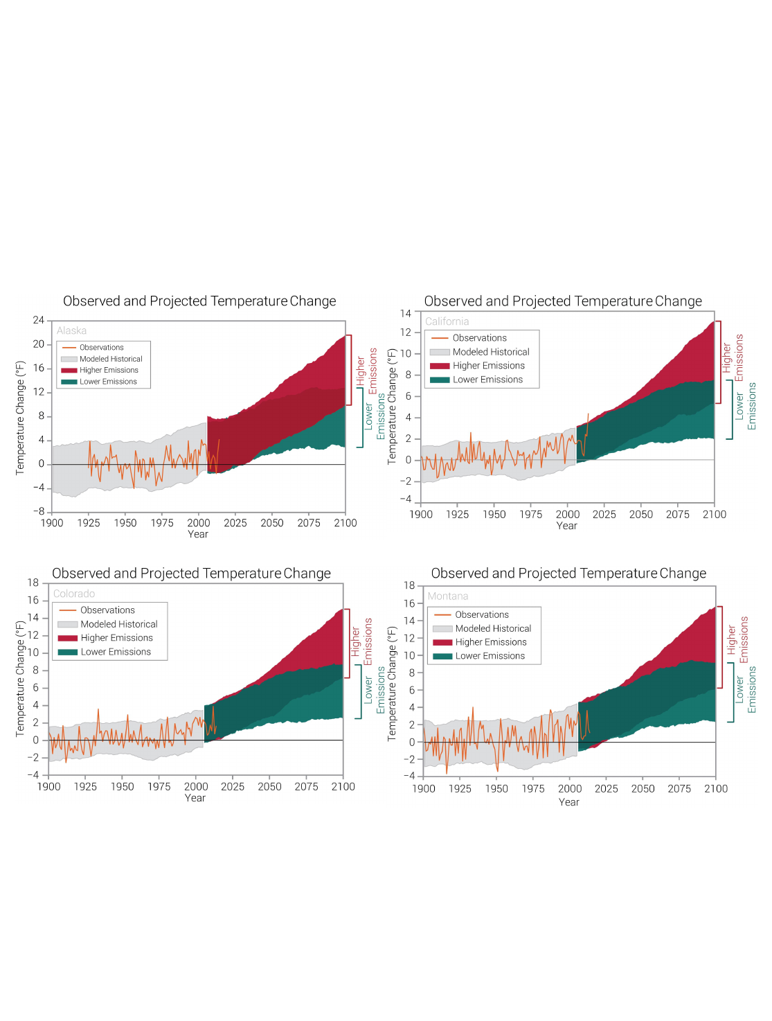
BLM 2021
Climate models suggest that winter and spring precipitation will increase, which combined with rising
temperatures will increase the average lowest elevation at which snow falls. This will increase the likelihood
that some of the precipitation events now occurring as snow will fall as rain instead, reducing water storage
in the snowpack, particularly at lower elevations. Higher spring temperatures will also result in earlier
melting of the snowpack, further decreasing water availability during the drier summer months. Heavier
spring precipitation, combined with a shift from snow to rain, could also increase the potential for flooding.
The intensity of future droughts is projected to increase. Even if precipitation amounts increase in the future,
temperature increases will intensify evaporation rates, resulting in lower soil moisture during dry spells.
Thus, future summer droughts, a natural part of the Wyoming climate, are likely to become more intense.
This in turn will increase the risk of wildfires, which are projected to become more frequent and severe.
Decreasing snowpack and earlier melt will have regional impacts as the state’s abundant snowfall feeds
major river systems in the United States.
(a) (b)
(c) (d)
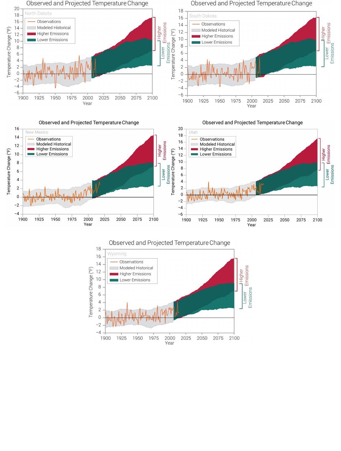
BLM 2021
(e) (f)
(g) (h)
(i)
Figure 9-3. Observed and Projected State Temperatures

BLM 2021
9.5 Effects on Public Health and Safety
The following data have been summarized from the Centers for Disease Control and Prevention, Climate and
Health website. Climate change and other natural and human-made health stressors influence human health
and disease in numerous ways. Some existing health threats will intensify, and new health threats will
emerge as a result of climate change. Key weather and climate drivers of health impacts include increasingly
frequent, intense, and longer lasting extreme heat, which worsen drought, wildfire, and air pollution risks;
increasingly frequent extreme precipitation, intense storms, and changes in precipitation patterns that lead to
drought and ecosystem changes; and rising sea levels that intensify coastal flooding and storm surges. Key
drivers of vulnerability include the attributes of certain groups (e.g., age, socioeconomic status, race, current
level of health) and of place (e.g., floodplains, coastal zones, urban areas), as well as the resilience of critical
public health infrastructure. Health effects of these disruptions include increased respiratory and
cardiovascular disease, injuries, and premature deaths related to extreme weather events, changes in the
prevalence and geographical distribution of foodborne and waterborne illnesses and other infectious
diseases, and threats to mental health.
Climate change is projected to affect human health by contributing to degrading air quality in many regions.
Increases in dust, pollen and allergens, wildfire smoke, and ground level ozone associated with changes in
climate are already being realized in the U.S. Atmospheric warming can increase the formation of ground
level ozone which is a GHG and adds to the heat trapping effect. Ground-level ozone (a key component of
smog) is associated with many health problems, such as diminished lung function, increases in
cardiovascular disease, and increases in premature deaths. Climate change effects including drought, heat
waves, and stagnation events can impact air quality causing increased concentrations of particulate matter.
Increases in wildfires and associated smoke, drier conditions that create more airborne dust, and changes in
vegetation that result in increases in pollen and allergens all contribute to increases in particulate matter in
the air. Health effects of particulate matter include asthma, heart disease, lung cancer, and other disease.
Climate change is currently increasing the vulnerability of many forests to wildfire. Climate change is
projected to increase the frequency of wildfires in certain regions of the United States. Long periods of
record high temperatures are associated with droughts that contribute to dry conditions and drive wildfires in
some areas. Wildfire smoke contains particulate matter, carbon monoxide, nitrogen oxides, and various
volatile organic compounds (i.e., ozone precursors) and can significantly reduce air quality locally and in
areas downwind of fires. Smoke exposure increases respiratory and cardiovascular hospitalizations,
emergency department visits, medical visits for lung illnesses, and medication dispensations for asthma,
bronchitis, chest pain, chronic obstructive pulmonary disease (COPD), and respiratory infections.
Drought conditions may increase environmental exposure to dust storms, extreme heat events, flash
flooding, degraded water quality, and reduced water quantity. Dust storms associated with drought
conditions contribute to degraded air quality. Extreme heat events have long threatened public health in the
United States. Heat waves are also associated with increased hospital admissions for cardiovascular, kidney,
and respiratory disorders. Extreme summer heat is increasing in the United States, and climate projections
indicate that extreme heat events will be more frequent and intense in coming decades.
Milder winters resulting from a warming climate can reduce illness, injuries, and deaths associated with cold
and snow. Vulnerability to winter weather depends on many nonclimate factors, including housing, age, and
baseline health. Although deaths and injuries related to extreme cold events are projected to decline due to
climate change, these reductions are not expected to compensate for the increase in heat-related deaths.

BLM 2021
The frequency of heavy precipitation events has already increased for the nation as a whole and is projected
to increase in all U.S. regions. Increases in both extreme precipitation and total precipitation have
contributed to increases in severe flooding events in certain regions. In addition to the immediate health
hazards associated with extreme precipitation events when flooding occurs, other hazards can often appear
once a storm event has passed. Elevated waterborne disease outbreaks have been reported in the weeks
following heavy rainfall, although other variables may also affect these associations. Water intrusion into
buildings can result in mold contamination that manifests later, leading to indoor air quality problems.
Buildings damaged during hurricanes are especially susceptible to water intrusion. Populations living in
damp indoor environments experience increased prevalence of asthma and other upper respiratory tract
symptoms, such as coughing and wheezing, as well as lower respiratory tract infections such as pneumonia,
respiratory syncytial virus (RSV), and RSV pneumonia.
Climate is one of the factors that influences the distribution of diseases borne by vectors such as fleas, ticks,
and mosquitoes, which spread pathogens that cause illness. The geographic and seasonal distribution of
vector populations, and the diseases they can carry, depend not only on climate but also on land use,
socioeconomic and cultural factors, pest control, access to health care, and human responses to disease
risk, among other factors. Daily, seasonal, or year-to-year climate variability can sometimes result in
vector/pathogen adaptation and shifts or expansions in their geographic ranges. North Americans are
currently at risk from numerous vector-borne diseases, including Lyme, dengue fever, West Nile virus, Rocky
Mountain spotted fever, plague, and tularemia. Vector-borne pathogens not currently found in the United
States, such as chikungunya, Chagas disease, and Rift Valley fever viruses, are also potential threats.
Mental illness is a major concern in the United States, and extreme weather events can affect mental health
in several ways. For example, research demonstrated high levels of anxiety and post-traumatic stress
disorder among people affected by Hurricane Katrina, and similar observations have followed floods and heat
waves. Some evidence suggests wildfires have similar effects. All of these events are increasingly fueled by
climate change. Additional potential mental health impacts, less well understood, include the possible
distress associated with environmental degradation and displacement, and the anxiety and despair that
knowledge of climate change might elicit in some people.
* * *

BLM 2021
Much of the current policy on mitigating emissions in the U.S. comes from individual states and
municipalities as well as market forcing that results when institutions move assets and future investments
away from fossil fuel projects. The BLM’s decision space for mitigating climate impacts from fossil fuel
development is currently limited by authorization in statutes such as FLPMA and the MLA. The BLM is
required to ensure its authorized activities follow the laws and regulations governing GHG emissions, prevent
undue waste of federal minerals, and promote efforts to minimize damage to the environment, in general.
This chapter discusses the options within BLM’s authority for mitigating the impacts of GHG emissions from
fossil fuels. Other applicable regulations that limit GHGs under the authority of other federal and state
agencies are discussed in Chapter 2.
No single authorized project level action can produce emissions with such significance that the action could
be perceived as influencing the climate. However, all GHG emissions (big and small) contribute to changes in
atmospheric radiative forcing and ultimately climate change. Even though climate change is a cumulative
phenomenon, a project's contribution to climate change can be limited as its net emissions are reduced, with
little or no contribution to climate change as net emissions approach zero. Net-zero emissions can be
achieved through a combination of controlling and offsetting emissions. Controls limit the amount of GHGs
that are emitted to the atmosphere, while offsets either remove GHGs from the atmosphere or reduce
emissions in other areas.
GHG emissions from individual BLM-approved actions may be subject to reductions or potential prevention
by selecting a reasonable alternative that responds to the action's purpose and need and applying
appropriate mitigation. Guidance on how to consider this in NEPA documents was presented in the CEQ’s
guidance dated August 1, 2016 entitled Final Guidance for Federal Departments and Agencies on
Consideration of Greenhouse Gas Emissions and the Effects of Climate Change in National Environmental
Policy Act Reviews (currently under review). However, the BLM has limited ability to provide for meaningful
or measurable mitigations actions in the context of cumulative climate change resulting from global
emissions. Indeed, as shown in Chapters 5 and 6, the production related emissions on the federal mineral
estate represent a small percentage of the U.S. and global emissions resulting from fossil fuel energy
demand.
10.1 Emissions Reduction Potential
The majority of GHG emissions resulting from federal fossil fuel authorizations occur outside of the BLM’s
authority and control. These emissions are referred to as indirect emissions and generally occur off-lease
during the transport, distribution, refining, and end-use of the produced federal minerals. The BLM’s decision
space for the downstream emissions is limited to either selecting the no action alternative (i.e., not
authorizing lands for fossil fuel development), or choosing alternatives with offsets for portions of the
emissions. The various strategies available to the BLM for offsetting emissions are subsequently described.
The BLM's decision authority primarily covers the direct or on-lease portions of natural gas and petroleum
systems. The BLM has developed best management practices (BMPs) designed to reduce emissions from
field production and operations for on-lease activities. BMPs may include limiting emissions on stationary
combustion sources, mobile combustion sources, fugitive sources, and process emissions occurring on a
lease parcel. Analysis and approval of future development on the lease parcels may include application of
10.0 Mitigation

BLM 2021
BMPs within the BLM’s authority, as conditions of approval, or controls, to reduce or mitigate GHG
emissions. Additional measures developed at the project development stage also may be incorporated as
applicant-committed measures by the project proponent or added to necessary air quality permits.
Mitigation measures to reduce direct GHG emissions from oil and gas operations may include the following:
Flare hydrocarbon and gases at high temperatures in order to reduce emissions of incomplete
combustion through the use of multichamber combustors.
Require that vapor recovery systems be maintained and functional in areas where petroleum liquids are
stored.
Install of liquids gathering facilities or central production facilities to reduce the total number of
sources and minimize truck traffic.
Use natural gas fired or electric drill rig engines.
Use selective catalytic reducers and low-sulfur fuel for diesel-fired drill rig engines.
Implement directional and horizontal drilling technologies whereby one well provides access to
petroleum resources that would normally require drilling several vertical wellbores.
Additionally, the BLM encourages oil and natural gas companies to adopt proven cost-effective technologies
and practices that improve operation efficiency and reduce natural gas emissions, to reduce the ultimate
impact from the emissions. The EPA reports that 89% of the CH reductions came from the oil and gas
production sector. By utilizing a variety of technologies including, reduced blow down frequency, installing
vapor recovery units, and converting gas-driven pumps to electric, mechanical, or solar driven pumps
operators can develop innovative project design features to self-limit their emissions. The BLM will continue
to work with industry to promote the use of the relevant BMPs for operations proposed on federal mineral
leases where such mitigation is consistent with agency authorities and policies.
10.2 Offsetting Emissions
In addition to controlling or preventing emissions, strategies to offset emissions could be utilized to align
BLM decisionmaking with the goal of achieving net-zero emissions by 2050. The following are various
strategies available to the BLM for offsetting emissions. These strategies may or may not be useful for
offsetting emissions from individual leases, and other carbon offset strategies may exist beyond those listed
here.
Carbon Sequestration
In 2018, the U.S. Geological Survey (USGS) produced a report estimating GHG emissions and sequestration
on Federal lands from 2005 to 2014. The report provides net ecosystem productivity (NEP) factors for all
federal lands in the United States. Net ecosystem productivity (NEP) is the amount of CO converted to fixed
carbon by the terrestrial ecosystem and is the product of CO converted to carbon through photosynthesis
minus the release of CO back into the atmosphere from plant respiration and the decomposition of dead
organic matter. The report also provided details on land use changes and land cover changes (LULC) which
are typically brought on by wildfires, harvest, and general land development. LULC reduces the effective rate
of NEP and is reported as net biome productivity (NBP). NBP is the final figure used in the USGS report to
calculate the net emissions between federal fossil fuel emissions and the sequestration capacity of the
federal lands. Here the BLM is attempting to do the same type of calculation for the report year emissions.
4
2
2
2

BLM 2021
Although the NBP data is a few years old and conditions on the ground may have changed in some regions of
the U.S., it is the best data available to show region-by-region sequestration and net emissions estimates. As
atmospheric concentrations of GHGs increase in the future, terrestrial ecosystems will generally sequester a
smaller percentage of emissions. Table 10-1 shows the average annual NEP and NBP from 2005 to 2014 and
average NEP and NBP per acre of land in different states and the nation. Averages of the datasets are
presented because factors such as wildfires can be highly variable between years. The negative values
indicate the sequestration capacity for the areas shown. At the national level, the USGS estimates that
terrestrial ecosystems (forests, grasslands, and shrublands) on federal lands sequestered an average of 195
Mt CO /yr between 2005 and 2014, offsetting approximately 15% of the CO emissions resulting from the
extraction of fossil fuels on federal lands and their end-use combustion. In the absence of site-specific data,
the average values per acre could be used to provide an estimate of sequestration for individual lease
parcels.
Table 10-1. Carbon Sequestration Capacity of Federal Lands (Mt CO e)
Federal Acres Source: Research Service 2020 report on Federal Land Ownership: Overview and Data
Historically, natural carbon sequestration in plants and soils has been able to lock up about 29% of all
anthropogenic emissions on a global scale. Natural sequestration is important because it offers a potential
path forward to help mitigate the impact of CO emissions and may play a long-term role in fighting climate
change. The Trillion Trees initiative is an example of an enhanced natural sequestration effort. This
multinational initiative seeks to reverse deforestation by planting and protecting one trillion trees by 2050.
The campaign claims that conserving intact forests, ending deforestation, and restoring trees and natural
ecosystems can provide about one-third of the solution to climate change by removing excess CO from the
atmosphere. Nationally, restoring forests and ecosystems devastated by wildfires could aid in this effort.
What remains unclear is how climate change will impact regional environments and their ability to sustain
historical or enhanced sequestration levels going forward.
2 2
2
State Federal Owned Acreage Mean NEP NEP per acre Mean NBP NBP per acre
Alaska 222,666,580 -63.7 -0.28608 -18 -0.08084
California 45,493,133 -30.67 -0.67417 -14.51 -0.31895
Colorado 24,100,247 -16.57 -0.68754 -13.84 -0.57427
Montana 27,082,401 -23.47 -0.86661 -18.85 -0.69602
New Mexico 24,665,774 -3.73 -0.15122 -2.15 -0.08717
North Dakota 1,733,641 -2.85 -1.64394 -1.82 -1.04981
Utah 33,267,621 -10.76 -0.32344 -8.58 -0.25791
Wyoming 29,137,722 -12.11 -0.41561 -10.39 -0.35658
Nationally 615,301,953 -342.93 -0.55734 -194.76 -0.31653
[42 ]
2
2

BLM 2021
Plugging Orphaned and Abandoned Wells
The EPA, in its "Inventory of U.S. GHG Emissions and Sinks" annual report, estimates that abandoned oil and
gas wells emitted 263,000 tonnes of CH and 7,000 tonnes of CO in 2019. Using AR5 GWPs, abandoned
wells emitted 7.4 Mt CO e in 2019. However, not all the wells classified as abandoned by the EPA are at the
end of their operational life. Some wells may be idled or shut-in and will return to production status, and
others may be turned into disposal wells. Plugging abandoned wells that are not expected to be used again
could reduce the overall emissions from federal lands.
There is limited emissions data to support emissions factors by oil and gas basin or production type. The
EPA uses information from the Townsend-Small et al. 2016 study which measured emissions from 138
abandoned wells in the Powder River Basin in Wyoming, Denver-Julesburg Basin in Colorado, Uintah Basin in
Utah, and Appalachian Basin in Ohio. The study authors developed emissions factors for well categories
observed to exhibit significantly different emissions levels: plugged versus unplugged (including inactive,
temporarily abandoned, shut in, dormant, orphaned, and abandoned), in eastern and western U.S. regions.
The authors used statistical bootstrapping on the data (sampled emissions rates) to provide factors with a
95% upper . Table 10-2 shows the emissions factors from the study. The unplugged wells
with the highest GHG emissions are found in the eastern U.S. with a mean emissions rate of 6.87 tonnes (t)
CO e/yr/well. Wells on federal land which are predominately in the western U.S. have a mean emissions rate
of 0.42 tonnes CO e/yr/well, which is 6% of the emissions of an unplugged well in the eastern U.S.
Table 10-2. Potential GHG Emissions from Orphaned and Abandoned Wells
Source: Townsend-Small et al. (2016)
Energy Substitution
Overall, GHG emissions could be reduced if fossil fuel energy production is avoided by substituting the use of
lower emitting forms of energy. The National Renewable Energy Laboratory (NREL) reviewed and
summarized life cycle assessment (LCA) emissions of different electricity generating technologies to reduce
4 2
2
[43 ]
confidence limit
2
2
Well Category
Mean
(g/hr/well)
95% Upper
Confidence
Limit (g/hr/well)
Mean (t
CO e/yr/well)
95% Upper
Confidence
Limit (t
CO e/yr/well)
2
2
All wells (entire U.S.) 1.38 3.17 0.34 0.78
All wells (eastern U.S.) 14 32.87 3.43 8.06
All wells (western U.S.) 0.18 0.41 0.04 0.10
Plugged wells (entire
U.S.)
0.00 0.01 0.00 0.00
Unplugged wells (entire
U.S.)
10.02 22.47 2.46 5.51
Plugged (eastern U.S.) 0 NA 0 NA
Unplugged (eastern U.S.) 28.01 64 6.87 15.7
Plugged (western U.S.) 0.00 0.01 0.00 0.00
Unplugged (western U.S.) 1.71 3.83 0.42 0.94

BLM 2021
uncertainties around estimates of environmental impacts and increase the value of the LCAs in
decisionmaking. The LCAs provided in Table 10-3 show the amount of GHG emissions from different types
of electrical grid energy sources. Even renewable energy sources, referred to as carbon neutral, emit some
GHGs during facility construction, maintenance, decommissioning, and from transportation and distribution
of energy. Of these energy sources, the BLM offers leases for coal, oil and gas, geothermal, wind, and solar.
Table 10-3. GHG Emission Factors for Comparison of Electrical System Energy Sources
Source: NREL
Over the past decade the energy sector has seen a decrease in annual GHG emissions as energy production
from coal has decreased while energy production from natural gas and renewables has increased. Over the
short term the trend of an increasing mix of natural gas and renewable energy production is expected to
continue, eventually transitioning to mostly renewables in the long term.
The BLM keeps statistics on the designed electric generating capacity of existing and pending wind, solar,
and geothermal projects on BLM-managed lands. A summary of the generating capacity for each renewable
is provided in Table 10-4. If the renewable projects replace existing fossil fuel energy production and reduce
the demand for federal fossil fuels, the potential foreseeable emissions reductions would range from 11.9 Mt
CO e for replacing Natural Gas energy production to 25.9 Mt CO e for replacing coal energy production.
Table 10-4. Electric Generating Capacity of Federal Lands
Source: https://www.blm.gov/programs/energy-and-minerals/renewable-energy
Carbon Capture
In addition to efforts to better respond and adapt to climate change, other federal initiatives are also being
implemented to mitigate climate change. The Carbon Storage Project was implemented to develop carbon
sequestration methodologies for geological (i.e., underground) and biological (e.g., forests and rangelands)
carbon storage. The project is a collaboration of federal and nonfederal stakeholders to enhance carbon
storage in geologic formations and in plants and soils in an environmentally responsible manner. The Carbon
Footprint Project is an effort to develop a unified GHG emission reduction program for the DOI, including
setting a baseline and reduction goal for the Department’s GHG emissions and energy use. Some research
Units Coal Natural Gas Biopower Geothermal Wind Solar Hydro Nuclear
grams CO e/kWh
2
980 465 40 11 - 47 11 27 - 44 7 12
2 2
Renewable
Source
Existing
Capacity
(Mega Watts)
Pending
Capacity
(Mega Watts)
Potential GHG
Reduction
Compared to Coal (Mt
CO e)
Potential GHG Reduction
Compared to Natural Gas (Mt
CO e)
2
2
Geothermal 1,235 727 6.07 2.79
Solar 2,656 1,380 11.52 5.29
Wind 1,088 993 8.29 3.81
Total 4,979 3,100 25.88 11.89

BLM 2021
has shown that coal-fired power plants using carbon capture and sequestration (CCS) technology can reduce
GHG emissions by approximately 80% compared to coal-fired power plants without CCS technology. While
CCS technology is still in the early adoption stage, it does show potential for reducing GHG emissions.
Another form of carbon capture includes recovering and using coal mine methane (CMM). The main idea
behind capturing CMM is to recover methane that would otherwise be released from a coal seam and leak
into the atmosphere. The recovered methane would then be combusted which converts the methane to
carbon dioxide and water, less potent GHGs. Technology is readily available to recover and use CMM.
Specific CMM end-uses depend on the gas quality, especially the concentration of methane and the presence
of contaminants. Worldwide, CMM is most often used for power generation, district heating, boiler fuel, or
town gas, or it is sold to natural gas pipeline systems.
Compensatory Mitigation
Compensatory mitigation is the process of offsetting adverse impacts by replacing or substituting the
affected resource or environment through a proponent’s offsite actions, monetary payments, or in-kind
contributions. Some examples of compensatory mitigation for GHG emissions include plugging orphaned
and abandoned wells, purchasing carbon offsets, or supporting land improvement projects that maximize
carbon sequestration. Prior BLM policy stated that compensatory mitigation could only be applied at the
development stage if the project proponent offered it as a component of a development plan or if it was
required by state or federal laws other than FLPMA (BLM Instruction Memorandum (IM) 2019-018,
"Compensatory Mitigation"). However, Secretarial Order (SO) 3398, "Revocation of Secretary’s Orders
Inconsistent with Protecting Public Health and the Environment and Restoring Science to Tackle the Climate
Crisis" (April 16, 2021), rescinded SO 3349, "American Energy Independence" (March 29, 2017), and SO 3360,
"Rescinding Authorities Inconsistent with Secretary’s Order 3349" (December 22, 2017), which IM 2019-018
was based, and the BLM issued IM-2021-038 on July 14, 2021, rescinding the previous IM-2019-018. The
BLM expects to establish policies which are aligned with EO 13990, SO 3398, and the priorities of the
Department. During this interim period offices should consider and implement compensatory mitigation on a
case-by-case basis, in consultation with state office and national office program specialists and the Office of
the Solicitor as needed.
* * *

BLM 2021
abandoned
- An oil or gas well is considered abandoned when it has been permanently taken out of
production.
actual fossil fuel production
- federal oil and gas lease that is considered to be in an “actual production”
status whenever it contains one or more wells drilled on a lease or agreement (communitization or
unitization) basis which are producing oil and/or gas in paying quantities. A lease is also considered to be in
“actual production” status whenever it contains one or more wells drilled on a lease or agreement basis,
which are capable of producing oil and/or gas in paying quantities even though production is not then
occurring (BLM Handbook H-3100-1, 'Oil and Gas Leasing').
albedo
- The fraction of light that is reflected by a body or surface. It is commonly used in astronomy to
describe the reflective properties of planets, satellites, and asteroids. It is also an important consideration in
climatology since recent albedo decreases in the Arctic have increased heat absorption at the surface.
anthropogenic
- relating to, or resulting from, the influence of human beings on nature.
applications for permit to drill (APDs)
- A revocable authorization to use public land for a specified purpose.
carbon dioxide equivalents (CO2e)
- A method to express the impact of each different greenhouse gas
(methane, nitrous oxide, etc.) in terms of the equivalent amount of CO emissions that would create the
same amount of warming of the atmosphere.
climate feedbacks
- Feedback in general is the process in which changing one quantity changes a second
quantity, and the change in the second quantity in turn changes the first. For example, a positive feedback in
global warming is the tendency of warming to increase the amount of water vapor in the atmosphere, which
in turn leads to further warming.
completions
- Well completion is the process of making a well ready for production (or injection) after drilling
operations are completed. This may include hydraulic fracturing.
confidence limit
- In statistics, a confidence interval is a type of estimate computed from the observed data.
This gives a range of values for an unknown parameter. The interval has an associated confidence level that
gives the probability with which an estimated interval will contain the true value of the parameter.
cryosphere
- The part of the earth's surface characterized by the presence of frozen water, including
mountain glaciers and continental ice sheets, seasonal snow and ice cover on land, and sea ice.
decline
- Once an oil and gas well has been completed (the process of making a well ready for production),
its maximum production level can be attained within days or weeks. After this level has been reached
(transient flow period), there is a decline in production usually caused by loss of reservoir pressure or
changing volumes of produced fluid. The rate of production decline is depicted by a decline curve. Decline
curves generally show the amount of oil or gas produced per unit of time, for many successive periods.
2
Glossary of Terms

BLM 2021
direct emissions
- GHG emissions that are emitted from the development of coal, oil and gas on the federal
mineral estate (i.e., onsite mining or upstream operations).
downstream
- Includes GHG emissions from refining, distributing, and retail of extracted minerals. This
includes oil refineries, gas processing plants, products distributors, and natural gas distribution companies.
Downstream emissions also include end uses such combustion of fuels (gasoline, diesel, etc.), plastics,
pharmaceuticals, natural gas, and propane.
estimated ultimate recovery (EUR)
- The estimated quantity of expected total production from an oil or gas
reserve or well. The EUR for a well is calculated as the sum of the observed monthly production values plus
the sum of the monthly production values estimated using the decline curve, starting the month after the last
observed production month through month 360 (30 years in total).
federal lands
- All lands and interests in lands owned by the United States which are subject to the mineral
leasing laws, including mineral resources or mineral estates reserved to the United States in the conveyance
of a surface or nonmineral estate (43 CFR §3160.0-5).
federal mineral estate
- The onshore subsurface mineral estate owned by the Federal government and
managed by the BLM, regardless of surface ownership.
fiscal year
- A one-year period that companies and governments use for financial reporting and budgeting.
The Federal government defines a fiscal year as the period between October 1st to September 30th.
fugitive emissions
- Emissions of greenhouse gases that are not produced intentionally by a stack or vent
and may include leaks from industrial sources and pipelines (IPCC, 2006).
held-by-production
- A provision in an oil or natural gas property lease that allows the lessee, generally an
energy company, to continue drilling activities on the property as long as it is economically producing a
minimum amount of oil or gas. The held-by-production provision thereby extends the lessee's right to operate
the property beyond the initial lease term.
indirect emissions
- GHG emissions that are a consequence of the produced fossil fuels but occur
downstream from the point of production on federal lands and/or are outside of BLM’s approval authority.
leases
- An authorization to possess and use public land for a period of time sufficient to amortize capital
investments in the land.
life-cycle assessment
- A methodology for assessing environmental impacts associated with all the stages
of the life cycle of a commercial product, process, or service. For instance, in the case of a manufactured
product, environmental impacts are assessed from raw material extraction and processing (cradle), through
the product's manufacture, distribution and use, to the recycling or final disposal of the materials composing
it (grave).
megajoules (MJ)
- A megajoule is a derived unit of energy in the International System of Units. One joule is
equal to the energy transferred to (or work done on) an object when a force of one newton acts on that object
in the direction of the force's motion through a distance of one meter, and thus a megajoule is one million
times greater.

BLM 2021
megatonnes
- A tonne; symbol: (t) is a metric unit of mass equal to 1,000 kilograms. It is also referred to as a
metric ton. It is equivalent to approximately 2,204.6 pounds, or 1.102 short tons (US). Mega is multiple of
10^6, and thus a Megatonne; symbol: (Mt), is equal to one million metric tons.
multiple use and sustained yield
- A combination of balanced and diverse resource uses that takes into
account the long-term needs of future generations for renewable and nonrenewable resources, including
recreation, range, timber, minerals, watershed, and wildlife and fish, along with natural scenic, scientific, and
historical values.
operators
- Any person or entity including but not limited to the lessee or operating rights owner, who has
stated in writing to the authorized officer that it is responsible under the terms and conditions of the lease
for the operations conducted on the leased lands or a portion thereof (43 CFR §3160.0-5).
parcels
- The name given to an area of land made available for competitive or noncompetitive leasing (BLM
Handbook H-3100-1, 'Oil and Gas Leasing').
plugged
- A well is plugged by setting mechanical or cement plugs in the wellbore at specific intervals to
prevent fluid flow.
producible well
- A well producing oil or gas, or if not producing oil or gas, a well either declared or capable of
being declared producing.
public lands
- Any land and interest in land owned by the United States within the several States and
administered by the Secretary of the Interior through the Bureau of Land Management, without regard to how
the United States acquired ownership, except (1) lands located on the Outer Continental Shelf; and (2) lands
held for the benefit of Indians, Aleuts, and Eskimos (43 U.S.C §1702, Federal Land Policy and Management
Act of 1976, Sec. 103 (e)).
reasonably foreseeable development scenario
- A technical report containing a long-term projection
(scenario) of a particular use of the public lands, in this case oil and gas exploration, development,
production, and reclamation activity (BLM Handbook H-1624-1, 'Planning for Fluid Mineral Resources').
snow-water equivalents
- April 1 snow-water equivalents (SWE) are used as a surrogate for the total
seasonal precipitation accumulation and for the maximum seasonal snowpack on the ground.
spud
- Spudding is the process of beginning to drill a well in the oil and gas industry.
stoichiometric
- Stoichiometry is the study of the quantitative relationships or ratios between two or more
substances undergoing a physical change or chemical change (chemical reaction).
teleconnections
- A weather pattern that refers to a recurring and persistent, large-scale pattern of pressure
and circulation anomalies that spans vast geographical areas. Thus, they are often the culprit responsible for
abnormal weather patterns occurring simultaneously over seemingly vast distances.
* * *

BLM 2021
[1]
BLM (Bureau of Land Management). 2020. Public Land Statistics 2019. Volume 204. U.S. Department of
the Interior, Bureau of Land Management, National Operations Center, Denver, CO.
[2]
Federal Register. 2012. Vol. 77, No. 159, Thursday, August 16, 2012. 40 CFR Parts 60 and 63. Oil and
Natural Gas Sector. New Source Performance Standards and National Emission Standards for Hazardous Air
Pollutants Review; Final Rule. pp. 49496,49534, and 49535.
[3]
ACS (American Chemical Society). 2021. It’s Water Vapor, Not the CO2. Website. American Chemical
Society, Washington, DC. https://www.acs.org/content/acs/en/climatescience/climatesciencenarratives/its-
water-vapor-not-the-co2.html.
[4]
EPA (Environmental Protection Agency). 2021. Overview of Greenhouse Gases. Website. U.S.
Environmental Protection Agency. https://www.epa.gov/ghgemissions/overview-greenhouse-gases.
[5]
NOAA Lindsey, R. 2020. Climate Change: Atmospheric Carbon Dioxide. U.S. Department of Commerce,
National Oceanic and Atmospheric Administration.
[6]
NOAA (National Oceanic and Atmospheric Administration). 2015. Ocean-Atmosphere CO2 Exchange.
Website. U.S. Department of Commerce, National Oceanic and Atmospheric Administration, Global Systems
Laboratory. https://sos.noaa.gov.
[7]
WMO (World Meteorological Organization). 2018 Unexpected Increases in Global Emissions of CFC-11.
WMO Greenhouse Gas Bulletin No. 14: 1-8.
[8]
IPCC (Intergovernmental Panel on Climate Change). 2013. Climate Change 2013: The Physical Science
Basis. New York, NY: Cambridge University Press.
[9]
Lenzen, M. 2008. Double-Counting in Life Cycle Calculations. Journal of Industrial Ecology 12 (4): 583-599.
[10]
Skone, T.J., G. Cooney, M. Jamieson, J. Marriott, M. Mutchek, and M. Krynock. 2016. Life Cycle Analysis
of Coal Exports from the Powder River Basin. U.S. Department of Energy, National Energy Technology
Laboratory.
[11]
Skone, T.J., G. Schivley, M. Jamieson, J. Marriott, G. Cooney, J. Littlefield, M. Mutchek, M. Krynock, and C.
Shih. 2018. Life Cycle Analysis: Supercritical Pulverized Coal (SCPC) Power Plants. U.S. Department of
Energy, National Energy Technology Laboratory.
[12]
Lattanzio, R.K. 2015. Life-Cycle Greenhouse Gas Assessment of Coal and Natural Gas in the Power
Sector. R44090, Version 3. Congressional Research Service.
[13]
Cohn, D. 2021. Planning for Coal Mine Closures in the Powder River Basin. Website. Sightline Institute.
https://www.sightline.org/2021/05/11/planning-for-coal-mine-closures-in-the-powder-river-basin/.
References

BLM 2021
[14]
West, B. 2021. Coal transported to the U.S. electric power sector declined by 22% in 2020. U.S. Energy
Information Administration, Independent Statistics and Analysis, Washington, DC.
[15]
BLM (Bureau of Land Management). 2021. Coal Data. Website. U.S. Department of the Interior, Bureau of
Land Management. https://www.blm.gov/programs/energy-and-minerals/coal/coal-data.
[16]
Cooney, G., M. Jamieson, J. Marriott, J. Bergerson, A. Brandt, and T.J. Skone. 2017. Updating the U.S. Life
Cycle GHG Petroleum Baseline to 2014 with Projections to 2040 Using Open-Source Engineering-Based
Models. Environmental Science and Technology 2017 (51): 977-987.
[17]
DOE (Department of Energy). 2021. Hydrogen Production: Natural Gas Reforming. Website. U.S.
Department of Energy, Office of Energy Efficiency and Renewable Energy, Washington, DC.
https://www.energy.gov/eere/fuelcells/hydrogen-production-natural-gas-reforming.
[18]
Littlefield, J., S. Roman-White, D. Augustine, A. Pegallapati, G.G. Zaimes, S. Rai, G. Cooney, and T.J.
Skone. 2019. Life Cycle Analysis of Natural Gas Extraction and Power Generation. U.S. Department of Energy,
National Energy Technology Laboratory, Pittsburgh, PA.
[19]
BLM (Bureau of Land Management). 2021. Oil and Gas Statistics. Website. U.S. Department of the
Interior, Bureau of Land Management. https://www.blm.gov/programs-energy-and-minerals-oil-and-gas-oil-
and-gas-statistics.
[20]
UNEP (United Nations Environment Programme). 2020. Emissions Gap Report 2020: Executive Summary.
United Nations Environment Programme, Nairobi, Kenya.
[21]
Crippa, M. D. Guizzardi, M. Muntean, E. Schaaf, E. Solazzo, F. Monforti-Ferrario, J.G.J. Olivier, and E.
Vignati. 2020. Fossil CO2 emissions of all world countries. Publications Office of the European Union,
Luxembourg.
[22]
IEA (International Energy Agency). 2021. Global Energy Review: C02 Emissions in 2020. Website.
International Energy Agency. https://www.iea.org/articles/global-energy-review-co2-emissions-in-2020.
[23]
CEQ (Council on Environmental Quality). 2021. Guidance on Consideration of Greenhouse Gases.
Website. Council on Environmental Quality. https://www.ceq.doe.gov/guidance/ceq_guidance_nepa-ghg.html.
[24]
Hausfather, Z. 2018. Analysis: Why the IPCC 1.5C report expanded the carbon budget. Carbon Brief.
https://www.carbonbrief.org/analysis-why-the-ipcc-1-5c-report-expanded-the-carbon-budget.
[25]
Meinshausen, M., S.C.B. Raper, and T.M.L. Wigley. 2011. Emulating coupled atmosphere-ocean and
carbon cycle models with a simpler model, MAGICC6 – Part 1: Model description and calibration.
Atmospheric Chemistry and Physics 11 (4): 1417-1456.
[26]
Robock, A. 2000. Volcanic eruptions and climate. Reviews of Geophysics 38 (2): 191-219.
[27]
Schmidt, H., et al. 2012. Solar irradiance reduction to counteract radiative forcing from a quadrupling of
CO2: Climate responses simulated by four earth system models. Earth System Dynamics 3 (1): 63-78.

BLM 2021
[28]
Cash, B.A., and N.J. Burls. 2019. Predictable and Unpredictable Aspects of U.S. West Coast Rainfall and
El Niño: Understanding the 2015/2016 Event. Journal of Climate 32 (10): 2843-2868.
[29]
AMS (American Meteorological Society). 2012. Glossary of Meteorology. American Meteorological
Society.
[30]
NASA (National Aeronautics and Space Administration). 2021. Climate Change: How Do We Know?
Website. NASA Jet Propulsion Laboratory, Earth Science Communications Team, CA.
https://climate.nasa.gov/evidence/.
[31]
Lindsey, R. 2020. Climate Change: Atmospheric Carbon Dioxide. U.S. Department of Commerce, National
Oceanic and Atmospheric Administration.
[32]
Bova, S., Y. Rosenthal, Z. Liu, S.P. Godad, and M. Yan. 2021. Seasonal origin of the thermal maxima at the
Holocene and the last interglacial. Nature 589 (2021): 548-553.
[33]
Vose, R.S., S. Applequist, M. Squires, I. Durre, M.J. Menne, C.N. Williams Jr., C. Fenimore, K. Gleason, and
D. Arndt. 2014. Improved Historical Temperature and Precipitation Time Series for U.S. Climate Divisions.
Journal of Applied Meteorology and Climatology 53 (5): 1232-1251.
[34]
Miller, A.J., D.R. Cayan, T.P. Barnett, N.E. Graham, and J.M. Oberhuber. 1994. The 1976-77 Climate Shift of
the Pacific Ocean. Oceanography 7 (1): 21-26.
[35]
Hartmann, B., and G. Wendler. 2005. The Significance of the 1976 Climate Shift in the Climatology of
Alaska. Journal of Climate 18 (22): 4825-4839.
[36]
Griffin, D., and K.J. Anchukaitis. 2014. How unusual is the 2012-2014 California drought? Geophysical
Research Letters 41 (24): 9017-9023.
[37]
Belmecheri, S., F. Babst, E.R. Wahl, D.W. Stahle, and V. Trouet. 2015. Multi-century evaluation of Sierra
Nevada snowpack. Nature Climate Change Vol. 6: 2-3.
[38]
Mote, P.W., S. Li, D.P. Lettenmaier, M. Xiao, and R. Engel. 2018. Dramatic declines in snowpack in the
western US. Climate and Atmoshperic Science 1 (2): 1-6.
[39]
Vose, R.S., D.R. Easterling, K.E. Kunkel, A.N. LeGrande, and M.F. Wehner. 2017. Temperature changes in
the United States. In: Climate Science Special Report: Fourth National Climate Assessment. pp. 185-206.
Wuebbles, D.J., D.W. Fahey, K.A. Hibbard, D.J. Dokken, B.C. Stewart, and T.K. Maycock (eds). U.S. Global
Change Research Program, Washington, DC.
[40]
Riahi, K., et al. 2017. The Shared Socioeconomic Pathways and their energy, land use, and greenhouse
gas emissions implications: An overview. Global Environmental Change 42 (2017): 153-168.
[41]
IPCC (Intergovernmental Panel on Climate Change). 2018. Summary for Policymakers. In: Global
Warming of 1.5° C. Special Report. Allen, M., et al. (eds). Intergovernmental Panel on Climate Change.
[42]
Vincent, C.H., L.A. Hanson, and L.F. Bermejo. 2020. Federal Land Ownership: Overview and Data. R42346.
Congressional Research Service.

BLM 2021
[43]
Townsend-Small, A., T.W. Ferrara, D.R. Lyon, A.E. Fries, and B.K. Lamb. 2016 Emissions of coalbed and
natural gas methane from abandoned oil and gas wells in the United States. Geophysical Research Letters 43
(5): 2283-2290.
* * *