National Water-Quality Assessment Program
Toxic Substances Hydrology Program
Mercury in Fish, Bed Sediment, and Water from
Streams Across the United States, 1998–2005
U.S. Department of the Interior
U.S. Geological Survey
Scientific Investigations Report 2009–5109
Cover:
Center: Wetland-basin stream site. (Photograph by Dennis A. Wentz, U.S. Geological Survey.)
Insets left to right:
Inset 1: Urban-basin stream site. (Photograph by Barbara C. Scudder, U.S. Geological Survey.)
Inset 2: Mined-basin stream site. (Photograph by Barbara C. Scudder, U.S. Geological Survey.)
Inset 3: Forested-basin stream site. (Photograph by Faith A. Fitzpatrick, U.S. Geological Survey.)
Inset 4: Agricultural-basin stream site. (Photograph by Barbara C. Scudder, U.S. Geological Survey.)
Mercury in Fish, Bed Sediment, and
Water from Streams Across the
United States, 1998–2005
By Barbara C. Scudder, Lia C. Chasar, Dennis A. Wentz, Nancy J. Bauch,
Mark E. Brigham, Patrick W. Moran, and David P. Krabbenhoft
National Water-Quality Assessment Program
Toxic Substances Hydrology Program
Scientific Investigations Report 2009-5109
U.S. Department of the Interior
U.S. Geological Survey
U.S. Department of the Interior
KEN SALAZAR, Secretary
U.S. Geological Survey
Suzette M. Kimball, Acting Director
U.S. Geological Survey, Reston, Virginia: 2009
For more information on the USGS—the Federal source for science about the Earth, its natural and living resources,
natural hazards, and the environment, visit http://www.usgs.gov or call 1-888-ASK-USGS
For an overview of USGS information products, including maps, imagery, and publications,
visit http://www.usgs.gov/pubprod
To order this and other USGS information products, visit http://store.usgs.gov
Any use of trade, product, or firm names is for descriptive purposes only and does not imply endorsement by the
U.S. Government.
Although this report is in the public domain, permission must be secured from the individual copyright owners to
reproduce any copyrighted materials contained within this report.
Suggested citation:
Scudder, B.C., Chasar, L.C., Wentz, D.A., Bauch, N.J., Brigham, M.E., Moran, P.W., and Krabbenhoft, D.P., 2009,
Mercury in fish, bed sediment, and water from streams across the United States, 1998–2005: U.S. Geological Survey
Scientific Investigations Report 2009–5109, 74 p.
iii
Foreword
The U.S. Geological Survey (USGS) is committed to providing the Nation with reliable scientific information
that helps to enhance and protect the overall quality of life and that facilitates effective management of water,
biological, energy, and mineral resources (http://www.usgs.gov/). Information on the Nation’s water resources
is critical to ensuring long-term availability of water that is safe for drinking and recreation and is suitable
for industry, irrigation, and fish and wildlife. Population growth and increasing demands for water make the
availability of that water, now measured in terms of quantity and quality, even more essential to the long-term
sustainability of our communities and ecosystems.
The USGS implemented the National Water-Quality Assessment (NAWQA) Program in 1991 to support
national, regional, State, and local information needs and decisions related to water-quality management and
policy (http://water.usgs.gov/nawqa). The NAWQA Program is designed to answer: What is the quality of our
Nation’s streams and groundwater? How are conditions changing over time? How do natural features and
human activities affect the quality of streams and groundwater, and where are those effects most pronounced?
By combining information on water chemistry, physical characteristics, stream habitat, and aquatic life, the
NAWQA Program aims to provide science-based insights for current and emerging water issues and priorities.
During 1991–2001, the NAWQA Program completed interdisciplinary assessments and established a baseline
understanding of water-quality conditions in 51 of the Nation’s river basins and aquifers, referred to as Study
Units (http://water.usgs.gov/nawqa/studyu.html).
National and regional assessments are ongoing in the second decade (2001–2012) of the NAWQA Program
as 42 of the 51 Study Units are selectively reassessed. These assessments extend the findings in the Study
Units by determining status and trends at sites that have been consistently monitored for more than a decade,
and filling critical gaps in characterizing the quality of surface water and groundwater. For example, increased
emphasis has been placed on assessing the quality of source water and finished water associated with many of
the Nation’s largest community water systems. During the second decade, NAWQA is addressing five national
priority topics that build an understanding of how natural features and human activities affect water quality,
and establish links between sources of contaminants, the transport of those contaminants through the
hydrologic system, and the potential effects of contaminants on humans and aquatic ecosystems. Included are
studies on the fate of agricultural chemicals, effects of urbanization on stream ecosystems, bioaccumulation
of mercury in stream ecosystems, effects of nutrient enrichment on aquatic ecosystems, and transport of
contaminants to public-supply wells. In addition, national syntheses of information on pesticides, volatile
organic compounds (VOCs), nutrients, trace elements, and aquatic ecology are continuing.
The USGS aims to disseminate credible, timely, and relevant science information to address practical and
effective water-resource management and strategies that protect and restore water quality. We hope this
NAWQA publication will provide you with insights and information to meet your needs, and will foster
increased citizen awareness and involvement in the protection and restoration of our Nation’s waters.
The USGS recognizes that a national assessment by a single program cannot address all water-resource
issues of interest. External coordination at all levels is critical for cost-effective management, regulation,
and conservation of our Nation’s water resources. The NAWQA Program, therefore, depends on advice
and information from other agencies—Federal, State, regional, interstate, Tribal, and local—as well as
nongovernmental organizations, industry, academia, and other stakeholder groups. Your assistance and
suggestions are greatly appreciated.
Matthew C. Larsen
Associate Director for Water
iv
This page intentionally left blank.
v
Contents
Foreword ........................................................................................................................................................iii
Abstract ..........................................................................................................................................................1
Introduction ....................................................................................................................................................1
Purpose and Scope ..............................................................................................................................2
Study Design ..........................................................................................................................................3
Methods...........................................................................................................................................................5
Field Data Collection.............................................................................................................................5
Ancillary Data Collection .....................................................................................................................6
Laboratory Analyses.............................................................................................................................8
Data Analyses........................................................................................................................................8
Quality Control .......................................................................................................................................9
Spatial Distribution of Mercury in Fish, Bed Sediment, and Stream Water .........................................9
Fish ..................................................................................................................................................10
Bed Sediment ......................................................................................................................................19
Stream Water ......................................................................................................................................23
Comparisons to Benchmarks and Guidelines .........................................................................................27
Comparisons Among Fish, Bed Sediment, and Stream Water .............................................................27
Comparisons Between Mined and Unmined Basins .............................................................................30
Factors Related to Mercury Bioaccumulation in Fish ...........................................................................32
Comparisons Among Land-Use/Land-Cover Categories .............................................................32
Fish Species-Specific Relations with Environmental Characteristics ......................................33
Bed-Sediment Relations with Environmental Characteristics ............................................................42
Stream-Water Relations with Environmental Characteristics ............................................................46
Discussion of Findings and Comparison with Other Studies ................................................................46
Summary and Conclusions .........................................................................................................................50
Acknowledgments .......................................................................................................................................51
References ....................................................................................................................................................51
Appendix 1. Definitions for variable abbreviations used in tables 5 and 6. ....................................72
vi
Figures
Figure 1. Map showing streams sampled for mercury, 1998–2005 ………………………… 4
Figure 2. Graph showing land-use/land-cover categories for basins sampled for mercury,
1998–2005, and for all U.S. stream basins ………………………………………… 5
Figure 3. Map showing sites in mined basins sampled for mercury, 1998–2005, and all
known gold and mercury production mining sites ……………………………… 7
Figure 4. Map showing spatial distribution of fish species most commonly
sampled for mercury, 1998–2005 ………………………………………………… 11
Figure 5. Map showing spatial distribution of total mercury concentrations in game fish,
1998–2005 ………………………………………………………………………… 13
Figure 6. Graph showing frequency distribution of total mercury concentrations in fish,
1998–2005 ………………………………………………………………………… 14
Figure 7. Map showing spatial distribution of length-normalized total mercury
concentrations in largemouth bass, 1998–2005 …………………………………… 15
Figure 8. Map showing spatial distribution of length-normalized total mercury
concentrations in smallmouth bass, 1998–2005 …………………………………… 16
Figure 9. Map showing spatial distribution of length-normalized total mercury
concentrations in rainbow-cutthroat trout, 1998–2005 …………………………… 17
Figure 10. Map showing spatial distribution for percentiles of length-normalized total
mercury concentrations in brown trout, 1998–2005 ……………………………… 18
Figure 11. Map showing spatial distribution of total mercury concentrations in bed
sediment, 1998–2005 ……………………………………………………………… 20
Figure 12. Graphs showing frequency distribution of mercury concentrations in
bed sediment, 1998–2005 ………………………………………………………… 21
Figure 13. Map showing spatial distribution of methylmercury concentrations in
bed sediment, 1998–2005 ………………………………………………………… 22
Figure 14. Map showing spatial distribution of total mercury concentrations in
unfiltered stream water,1998–2005 ……………………………………………… 24
Figure 15. Graphs showing frequency distribution of mercury concentrations
in unfiltered water, 1998–2005 …………………………………………………… 25
Figure 16. Map showing spatial distribution of methylmercury concentrations in
unfiltered stream water, 1998–2005 ……………………………………………… 26
Figure 17. Boxplot showing statistical distributions of mercury concentrations in fish,
bed sediment, and water, 1998–2005 ……………………………………………… 28
Figure 18. Boxplots showing statistical distributions of mercury concentrations in bed
sediment and unfiltered water at stream sites in mined and unmined basins,
1998–2005 ………………………………………………………………………… 31
Figure 19. Boxplot showing statistical distributions of length-normalized mercury
concentrations in largemouth bass for U.S. streams draining various
land-use/land-cover categories, 1998–2005 ……………………………………… 32
vii
Figures—Continued
Figure 20. Redundancy Analysis (RDA) showing relative importance of selected
environmental characteristics (blue arrows and labels) to concentrations
of mercury in largemouth bass (green arrows and labels), 1998–2005 …………… 35
Figure 21. Graph showing correlations between length-normalized mercury
concentrations in fish and selected environmental characteristics, 1998–2005 … 36
Figure 22. Graphs showing Biota Accumulation Factors (BAF) for fish in relation to
selected environmental characteristics, 1998–2005 ……………………………… 41
Figure 23. Graphs showing correlations between mercury in bed sediment and
selected environmental characteristics in unmined basins, 1998–2005 ………… 43
Figure 24. Graphs showing correlations between mercury in unfiltered water and
selected environmental characteristics in unmined basins, 1998–2005 ………… 47
Tables
Table 1. Number of sites on United States streams sampled for mercury, 1998–2005 …… 3
Table 2. Summary of fish species sampled for mercury in U.S. streams, 1998–2005 ……… 10
Table 3A. Summary statistics for mercury in U.S. streams, 1998–2005:
Total mercury in fish ……………………………………………………………… 12
Table 3B. Summary statistics for mercury in U.S. streams, 1998–2005: Total and
methylmercury and ancillary chemical characteristics of bed sediment ………… 19
Table 3C. Summary statistics for mercury in U.S. streams, 1998–2005: Total and
methylmercury and ancillary water quality characteristics of unfiltered
stream water. ……………………………………………………………………… 23
Table 4A. Summary statistics for mercury Biota Accumulation Factors (BAFs) for fish
from U.S. streams, 1998–2005: BAFs for fish with respect to water and bed
sediment, all species ……………………………………………………………… 28
Table 4B. Summary statistics for mercury Biota Accumulation Factors (BAFs) for fish
from U.S. streams, 1998–2005: BAFs for fish with respect to water, individual
species …………………………………………………………………………… 29
Table 4C. Summary statistics for mercury Biota Accumulation Factors (BAFs) for fish
from U.S. streams, 1998–2005: BAFs for fish with respect to bed sediment,
individual species ………………………………………………………………… 30
Table 5. Spearman rank correlation coefficients (r
s
) for relations between
length-normalized total mercury in composite samples of fish and selected
environmental characteristics for U.S. streams, 1998–2005 ……………………… 34
Table 6. Spearman rank correlation coefficients (r
s
) for relations between selected
environmental characteristics from U.S. streams, 1998–2005 …………………… 44
Table 7. Land-use/land-cover characterization of U.S. streams sampled for mercury,
1998–2005 ………………………………………………………………………… 59

viii
Conversion Factors
Multiply By To obtain
Length
nanometer (nm) 0.00000003937 inch (in.)
micrometer (µm) 0.00003937 inch (in.)
millimeter (mm) 0.03937 inch (in.)
centimeter (cm) 0.3937 inch (in.)
meter (m) 3.281 foot (ft)
meter (m) 1.094 yard (yd)
kilometer (m) 0.6214 mile (mi)
Volume
liter (L) 0.2642 gallon (gal)
liter (L) 33.82 ounce, fluid (fl. oz)
Area
square meter (m
2
) 10.76 square foot (ft
2
)
square kilometer (km
2
) 0.3861 square mile (mi
2
)
Mass
gram (g) 0.03527 ounce, avoirdupois (oz)
kilogram (kg) 2.205 pound avoirdupois (lb)
Temperature in degrees Celsius (°C) may be converted to degrees Fahrenheit (°F) as follows:
°F=(1.8×°C)+32.
Concentrations of chemical constituents in water are given either in milligrams per liter
(mg/L), micrograms per liter (µg/L), or nanograms per liter (ng/L). Concentrations of chemical
constituents in fish tissue are given in micrograms per gram (µg/g); those in sediment are given
in nanograms per gram (ng/g).
Mercury in Fish, Bed Sediment, and Water from Streams
Across the United States, 1998–2005
By Barbara C. Scudder, Lia C. Chasar, Dennis A. Wentz, Nancy J. Bauch, Mark E. Brigham, Patrick W. Moran,
and David P. Krabbenhoft
Abstract
Mercury (Hg) was examined in top-predator sh, bed
sediment, and water from streams that spanned regional and
national gradients of Hg source strength and other factors
thought to inuence methylmercury (MeHg) bioaccumulation.
Sampled settings include stream basins that were agricultural,
urbanized, undeveloped (forested, grassland, shrubland, and
wetland land cover), and mined (for gold and Hg). Each site
was sampled one time during seasonal low ow. Predator
sh were targeted for collection, and composited samples
of sh (primarily skin-off llets) were analyzed for total Hg
(THg), as most of the Hg found in sh tissue (95–99 percent)
is MeHg. Samples of bed sediment and stream water were
analyzed for THg, MeHg, and characteristics thought to
affect Hg methylation, such as loss-on-ignition (LOI, a
measure of organic matter content) and acid-volatile sulde
in bed sediment, and pH, dissolved organic carbon (DOC),
and dissolved sulfate in water. Fish-Hg concentrations at 27
percent of sampled sites exceeded the U.S. Environmental
Protection Agency human-health criterion of 0.3 micrograms
per gram wet weight. Exceedances were geographically
widespread, although the study design targeted specic
sites and sh species and sizes, so results do not represent
a true nationwide percentage of exceedances. The highest
THg concentrations in sh were from blackwater coastal-
plain streams draining forests or wetlands in the eastern and
southeastern United States, as well as from streams draining
gold- or Hg-mined basins in the western United States (1.80
and 1.95 micrograms THg per gram wet weight, respectively).
For unmined basins, length-normalized Hg concentrations
in largemouth bass were signicantly higher in sh from
predominantly undeveloped or mixed-land-use basins
compared to urban basins. Hg concentrations in largemouth
bass from unmined basins were correlated positively with
basin percentages of evergreen forest and also woody wetland,
especially with increasing proximity of these two land-
cover types to the sampling site; this underscores the greater
likelihood for Hg bioaccumulation to occur in these types
of settings. Increasing concentrations of MeHg in unltered
stream water, and of bed-sediment MeHg normalized by LOI,
and decreasing pH and dissolved sulfate were also important
in explaining increasing Hg concentrations in largemouth bass.
MeHg concentrations in bed sediment correlated positively
with THg, LOI, and acid-volatile sulde. Concentrations of
MeHg in water correlated positively with DOC, ultraviolet
absorbance, and THg in water, the percentage of MeHg in bed
sediment, and the percentage of wetland in the basin.
Introduction
Mercury (Hg) is a global pollutant that ultimately makes
its way into every aquatic ecosystem through the hydrologic
cycle. Anthropogenic (human-related) sources are estimated
to account for 50–75 percent of the annual input of Hg to the
global atmosphere and, on average, 67 percent of the total Hg
in atmospheric deposition to the United States (Meili, 1991;
U.S. Environmental Protection Agency, 1997; Seigneur and
others, 2004). Elevated Hg concentrations that are attributed
to atmospheric deposition have been documented worldwide
in aquatic ecosystems that are remote from industrial sources
(Fitzgerald and others, 1998).
Methylation—the microbially mediated conversion of
inorganic Hg to the organic form, methylmercury (MeHg)—is
the single most important step in the environmental Hg cycle
because it greatly increases Hg toxicity and bioaccumulation
potential. Laboratory studies estimate the bioaccumulation
potential for MeHg to be a thousand-fold that of inorganic
Hg (Ribeyre and Boudou, 1994). In aquatic ecosystems,
MeHg is found in elevated concentrations in top predators,
and physiological effects have been demonstrated at low
concentrations (Briand and Cohen, 1987; Eisler, 1987; Wiener
and Spry, 1996; U.S. Environmental Protection Agency, 2001;
Rumbold and others, 2002; Tchounwou and others, 2003;
Yokoo and others, 2003; Eisler, 2004). The process by which
Hg is accumulated into the lower trophic levels of aquatic
food webs is not well understood (Wiener and others, 2003).
Although diet has been demonstrated to be the dominant
mechanism of MeHg uptake in sh (Hall and others, 1997),
factors such as size, age, community structure, feeding habits,
and food-chain length are also important in the ultimate MeHg
sh-tissue concentration (Wong and others, 1997; Atwell and
others, 1998; Trudel and others, 2000; Wiener and others,
2003).

2 Mercury in Fish, Bed Sediment, and Water from Streams Across the United States, 1998–2005
Accumulation of MeHg in sh tissue is considered a
signicant threat to the health of both wildlife and humans.
Approximately 95 percent or more of the Hg found in most
sh llet/muscle tissue is MeHg (Huckabee and others, 1979;
Grieb and others, 1990; Bloom 1992). Women of child-bearing
age and infants are particularly vulnerable to effects from
consumption of Hg-contaminated sh (U.S. Environmental
Protection Agency, 2001). As of 2006, most States (48; no
advisories in Alaska or Wyoming), the District of Columbia,
one territory (American Samoa), and two Tribes have issued
sh-consumption advisories for Hg (U.S. Environmental
Protection Agency, 2007). These advisories represent
14,177,175 lake acres and 882,963 river miles, or 35 percent
of the Nation’s total lake acreage and about 25 percent of its
river miles.
Studies of Hg in aquatic environments have focused
mostly on lakes, reservoirs, and wetlands because of the
predominance of lakes with Hg concerns and the importance
of wetlands in Hg methylation (Bloom and others, 1991;
Driscoll and others, 1994; Hurley and others, 1995;
Krabbenhoft and others, 1995; St. Louis and others, 1994
and 1996; Westcott and Kalff, 1996; U.S. Environmental
Protection Agency, 1997; Fitzgerald and others, 1998;
Kotnik and others, 2002). Increasingly, however, studies
of streams and rivers have contributed signicantly to our
understanding of Hg in these complex ecosystems (Hurley
and others, 1995; Balogh and others, 1998; Domagalski, 1998;
Wiener and Shields, 2000; Peckenham and others, 2003;
Dennis and others, 2005). Sources of regional or national
sh-Hg data include a U.S. Environmental Protection Agency
(USEPA) assessment of sh-Hg concentrations in streams
in the western United States (Peterson and others, 2007);
the USEPA National Lake Fish Tissue Studies (http://www.
epa.gov/waterscience/sh/study/); the National Contaminant
Biomonitoring Program (NCBP) of the U.S. Fish and
Wildlife Service, which later became the Biomonitoring of
Environmental Status and Trends (BEST) program of the
U.S. Geological Survey (USGS) (Schmitt and others, 1999,
2002 and 2004; Hinck and others, 2004a, 2004b, 2006, 2007);
sh-Hg data compiled from 24 research and monitoring
programs in northeastern North America (Kamman and others,
2005); and a large compilation of many State, Federal, and
Tribal sh-Hg datasets (Wente, 2004; see also http://emmma.
usgs.gov/datasets.aspx).
Currently, it is difcult to directly compare sh-Hg
concentrations across the Nation by using any compilation
of sh-Hg data. Several issues must be resolved before
making effective use of other agencies’ datasets, and review
of other-agency data is beyond the scope of this report. These
issues include (1) use of multiple analytical laboratories and
analytical methods; (2) inconsistent or unknown data quality;
(3) large variations in sample characteristics, including
sh species, size, and tissue sampled; (4) incomplete site
information (for example, locations of some sites are not
adequately described, and some georeferenced sites may not
be coded as to site type, such as lake, stream, or reservoir);
and (5) incomplete sample information (for example, species,
length, or tissue sampled are not known). Several of these
issues have been described in greater detail by Wente (2004),
who has developed a promising statistical modeling approach
to account for variation in sh-Hg levels by species, size,
and tissue sampled. It is not known, however, whether the
approach performs equally well in streams as it does in lakes,
or whether it performs consistently among various regions of
the Nation. These issues emphasize the need for a nationwide
assessment of Hg in streams for sh, bed sediment, and water
based on consistent methods, as is provided by the study
described herein.
Purpose and Scope
The primary objective of this report is to describe the
occurrence and distribution of total mercury (THg) in sh
tissue in streams in relation to regional and national gradients
of Hg source strength (including atmospheric deposition,
gold and Hg mining, urbanization) and other factors that are
thought to affect Hg bioaccumulation, including wetland and
other land-use/land-cover types (LULC). Secondary objectives
are to evaluate THg and MeHg in streambed (bed) sediment
and stream water in relation to these gradients and to identify
ecosystem characteristics that favor the production and
bioaccumulation of MeHg.
The data discussed here are presented by Bauch and
others (2009). They were aggregated from 6 studies covering
a total of 367 sites across the Nation (table 1). The majority
of sites (266) were part of 2 studies conducted collaboratively
by the USGS National Water-Quality Assessment (NAWQA)
and Toxics Substances Hydrology Programs. The earliest of
these, the USGS National Mercury Pilot Study (Krabbenhoft
and others, 1999; Brumbaugh and others, 2001) sampled 107
streams across the Nation in 1998. During 2002 and 2004–5,
an additional 159 streams were sampled by the NAWQA
Program to complement those sampled during the 1998
National Mercury Pilot Study; the additional sampling sites
were chosen to increase spatial coverage and to supplement
source and environmental factors that previously were
underrepresented. An additional 101 stream sites were
sampled as part of 4 regional USGS studies in the Cheyenne-
Belle Fourche River Basins, 1998–99 (S.K. Sando, USGS,

Introduction 3
unpublished data, 2005); Delaware River Basin, 1999–2001
(Brightbill and others, 2003); New England Coastal Basins,
1999–2000 (Chalmers and Krabbenhoft, 2001); and the Upper
Mississippi River Basin, 2004 (Christensen and others, 2006).
The regional studies used sample-collection, processing, and
analytical techniques that were comparable to those in the
two national studies, thus allowing direct comparison of the
results.
Study Design
Sampled streams were predominantly within the
boundaries of NAWQA study areas, which are major
hydrologic basins (g. 1). These major hydrologic basins
encompass 45 percent of the land area of the conterminous
United States, some portion of each of the 50 States, and
60–70 percent of water use and population served by public
water supply (Leahy and others, 1990; Helsel, 1995; Gilliom
and others, 2001); they represent broad ranges of hydrologic
and geologic settings, LULC, and population density. Within
each major basin, streams were selected to represent the
specic environmental settings of interest. The resulting
network of sites reects conditions across the United States.
Gilliom and others (1995), Helsel (1995), and Horowitz and
Stephens (2008) discuss the advantages of the NAWQA design
for sampling small streams at a national scale.
Specic site-selection criteria within each of the major
hydrologic basins were based on targeted environmental
settings thought to be important with regard to the source,
concentration, or biogeochemical behavior of Hg in aquatic
ecosystems in that basin (table 7, at back of report). Settings
of particular interest included agricultural areas (enhanced
runoff of dissolved and colloidal Hg associated with organic
matter; particulate Hg from eroded soils); urban areas
(elevated local depositional sources; enhanced Hg runoff due
to impervious surfaces); undeveloped areas (atmospheric Hg
deposition source only); and mined areas (cinnabar mining;
historical gold mining, in which elemental Hg was used
as an amalgamating agent). Site categories of agricultural,
urban, undeveloped, and mixed LULC are consistent with the
denitions provided by Gilliom and others (2006):
• Agricultural basins contained greater than 50 percent
agricultural land and less than or equal to 5 percent
urban land.
• Urban basins contained greater than 25 percent urban
land and less than or equal to 25 percent agricultural
land.
• Undeveloped basins were primarily forest, herbaceous
grassland, shrubland, tundra, and wetland, and
contained less than or equal to 5 percent urban land
and less than or equal to 25 percent agricultural land.
• Mixed-land-use basins included all remaining LULC
combinations.
Compared with all streams in the conterminous United States,
this targeted sampling for Hg may have overrepresented urban
basins and underrepresented undeveloped basins (g. 2).
Slightly more than two-thirds of the sampled Hg sites were
in the eastern half of the United States compared with the
western half (west of the Mississippi River).
Each site was sampled one time, typically during seasonal
low ow in late summer, for Hg and related constituents in
top-predator (piscivorous) sh, bed sediment, and stream
water. This multimedia approach on a national scale was
considered to be critical for helping to understand controls
on Hg partitioning, bioaccumulation, and biomagnication
(Krabbenhoft and others, 1999). Many studies have shown
that mature top-predator sh generally reect the highest
potential Hg concentrations in aquatic food webs (Francesconi
and Lenanton, 1992; Weiner and Spry, 1996; Boudou and
Ribeyre, 1997; Morel and others, 1998; Kim and Burggraaf,
1999). Thus, largemouth bass was the piscivorous sh species
targeted for collection. At sites where this species was not
available in sufcient numbers, alternate top-predator sh
species were collected.
Table 1. Number of sites on United States streams sampled for
mercury, 1998–2005.
[Regional studies: CHEY, Cheyenne-Belle Fourche River Basins, 1998–99;
DELR, Delaware River Basin, 1999–2001; NECB, New England Coastal
Basins, 1999–2000; and UMIS, Upper Mississippi River Basin, 2004]
Description
Number of
sites
Study components
1998 National Mercury Pilot Study 107
2002–05 Additional national studies 159
Regional studies: CHEY, DELR, NECB, UMIS 101
Total number of sites 367
Mercury data available
Fish mercury data 291
Bed-sediment and water mercury data 352
Fish, bed-sediment, and water mercury data 274
4 Mercury in Fish, Bed Sediment, and Water from Streams Across the United States, 1998–2005
11-7093_fig 01
0
250 500
MILES
0
250 500
KILOMETERS
0 100 200 MILES
0 100 200 KILOMETERS
0 500 1,000 MILES
0 500 1,000 KILOMETERS
0 50 100 MILES
0 50 100
KILOMETERS
100°
90°
80°
70°
110°
120°
30°
40°
40°
30°
75°
70°
45°
40°
155°160°
22°
19°
70°
130°150°170°W170°E
50°
60°
150° 140° 130°160°170°180°
50°
60°
70°
EXPLANATION
Studies
1998 National Mercury Pilot Study
2002–5 studies
CHEY-regional study
DELR-regional study
NECB-regional study
UMIS-regional study
NAWQA study area
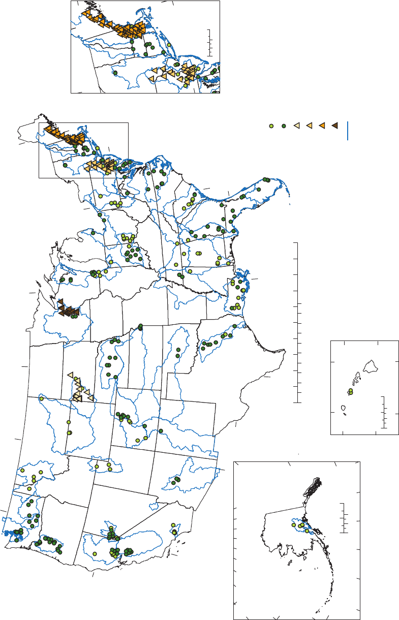
Figure 1. Streams sampled for mercury, 1998–2005. (Regional studies are: CHEY, Cheyenne-Belle Fourche River Basins, 1998–9; DELR, Delaware River Basin,
1999–2001; NECB, New England Coastal Basins, 1999–2000; and UMIS, Upper Mississippi River Basins, 2004.)

Methods 5
11-7093-c Mercury SIR_fig 02
0
10
20
30
40
50
60
70
Hg sampling sites U.S. streams
PROPORTION OF BASINS, IN PERCENT
Agricultural
Urban
Undeveloped
Mixed
Figure 2. Land-use/land-cover
categories for basins sampled for
mercury, 1998–2005, and for all U.S.
stream basins.
Methods
Methods for eld data collection, ancillary data
collection, laboratory analyses, and quality control are
summarized below and described in detail elsewhere
(primarily in Bauch and others, 2009; see also Lewis and
Brigham, 2004; Lutz and others, 2008; Scudder and others,
2008). All data presented in this report are published in Bauch
and others (2009).
Field Data Collection
Fish were collected primarily by electroshing, but
also by rod/reel and gill nets. Largemouth bass (3-year age
class) were targeted for collection; alternate top predators
were selected if largemouth bass were not available. Fish
were measured for total length and weight. Fish axial muscle,
primarily skinless llet (skin-on llet at four sites in the Upper
Mississippi River Basin regional study), was dissected from
most sh in the eld or laboratory by use of trace-metal clean
procedures (Scudder and others, 2008). Fish weighing less
than about 60 g were processed as whole-body or headless
sh (15 sites). For all samples except those collected during
2004–5, 1 to 10 sh (median of 5 sh) of the same species
and similar size for a site were composited to form a single
composite sample for analysis of THg. Fish collected during
2004–5 were processed individually for laboratory analyses.
After processing, sh samples were frozen until analysis.
Fish were not collected in the Cheyenne-Belle Fourche River
Basins.
Bed-sediment samples were collected by use of trace-
metal clean sampling techniques (Shelton and Capel, 1994;
Lutz and others, 2008). A Teon
®
or plastic scoop was used
to remove the upper 2 to 4 cm of bed sediment from 5 to 10
depositional areas; samples were composited in Teon
®
or
plastic containers into a single sample for each site. Each
sample was homogenized and subsampled for THg and MeHg,
loss-on-ignition (LOI, a measure of organic matter content),
acid-volatile sulde (AVS), and sand/silt particle size (percent
less than 63 µm) analyses. Samples were unsieved, so as to
minimize disturbance of the natural partitioning of MeHg
and THg in the bed sediment and volatilization of suldes.
Subsamples for Hg analysis were placed in Teon
®
vials and
frozen.
Stream-water samples were collected by dipping Teon
®
or PETG (Nalgene) bottles in the centroid of streamow
by use of trace-metal clean techniques (Olson and DeWild,
1999; Lewis and Brigham, 2004). Unltered THg samples
were acidied to 1 percent HCl by volume; unltered MeHg
samples were stored in a dark cooler until frozen (Krabbenhoft
and others, 1999). Samples for ltered THg and MeHg
analyses were passed through quartz ber lters (47-mm
diameter, 0.7-µm pore size) in the eld, placed into Teon
®
bottles, acidied to 1 percent HCl by volume, and stored in
the dark. Filters were placed on dry ice and stored frozen
until analysis of particulate THg and MeHg. Samples were
collected for additional water-quality characteristics, such
as pH, specic conductance, ultraviolet (UV) absorbance,
specic UV absorbance (SUVA) at 254 nanometers (nm),
and concentrations of dissolved organic carbon (DOC),
sulfate, and suspended sediment (total suspended sediment
concentration and fraction less than 63 µm). Streamow was
measured one time during Hg sampling at sites without stream
gages.

6 Mercury in Fish, Bed Sediment, and Water from Streams Across the United States, 1998–2005
Ancillary Data Collection
A detailed description of selected ancillary spatial data
for each stream basin is given in Bauch and others (2009).
Stream-basin boundaries were delineated by using 1:24,000-
to 1:250,000-scale digital topographic and hydrologic
maps (Nakagaki and Wolock, 2005) or 30-m resolution
Elevation Derivatives for National Applications (EDNA)
reach catchments (U.S. Geological Survey, 2002). To verify
accuracy, additional independent checks were made of
selected basin boundaries. Natural features and potential
human inuences within the study basins were characterized
by using Geographic Information System (GIS) coverages.
LULC information was obtained from 30-m resolution
National Land Cover Data (NLCD) that were based on
satellite imagery from the early to mid-1990s (Vogelmann
and others, 2001) and modied and enhanced (NLCDe 92)
with Geographic Information Retrieval and Analysis System
(GIRAS) data to give 25 LULC categories, as described in
Nakagaki and Wolock (2005). These were the most up-to-
date, nationally consistent LULC data at the time of our
analysis. All LULC values used in our report are percentages
of total basin area. Four initial groupings of sites were based
on criteria in Gilliom and others (2006): agricultural, urban,
undeveloped, and mixed. To address the possibility that
conditions observed at the sampling site were inuenced more
by LULC closer to the site than by LULC farther from the site,
LULC percentages were weighted by the inverse Euclidean
distance from the site and reported as distance-weighted
LULC. This resulted in a basin-scale percentage for each
LULC category that was adjusted for spatial proximity to the
sampling site; an area of a particular LULC category that was
closer to the site received a higher weight and value than an
area farther away (Wente, 2000; Falcone and others, 2007).
Gold and Hg mining can result in signicant
contributions of Hg to aquatic systems, so it was important
to characterize sites with regard to this particular land use.
Potential sources of Hg from past or current mining operations
were determined for each stream basin by using the Mineral
Availability System/Mineral Industry Location System (MAS/
MILS) database from the Bureau of Mines (V.C. Stephens,
U.S. Geological Survey, written commun., 2004), which is
now part of the Mineral Resources Data System (MRDS) of
the USGS (U.S. Geological Survey, 2004). The sites were
identied as (1) Hg mining operations, in general, (2) Hg
“producers,” (3) gold mining operations, in general, and
(4) gold “producers.” Producers included current or past
production mining operations. The highest densities of gold
or Hg production mining sites are in Arkansas, California,
Colorado, Idaho, Montana, and Nevada. A total of 89 basins
were designated as “mined” and treated separately for the
purposes of our data analyses; however, this distinction
was made only for data analyses in our report and does not
necessarily imply impacts of mining in these basins (g. 3).
In addition, our study was not designed specically to address
impacts of mining, so there may be areas of intense gold and
Hg mining that were not represented. Mined basins in the
eastern United States represented only gold mining.
Key soil characteristics were compiled from the U.S.
Department of Agriculture State Soil Geographic (STATSGO)
database (U.S. Department of Agriculture, 1994). Percent
organic matter, soil erodibility factor, and land-surface slope
were from Wolock (1997) and were linked by mapping-unit
identication code to a 100-m resolution national grid of
STATSGO geographic mapping units.
Basin hydrologic data were derived from various sources.
Mean annual precipitation is the average value predicted
from the Parameter-elevation Regressions on Independent
Slopes Model (PRISM) (Daly, Neilson, and Phillips, 1994;
Daly, Taylor, and Gibson, 1997) based on annual precipitation
(1961–90) at 2-km resolution obtained from the Spatial
Climate Analysis Service at Oregon State University,
Corvallis, Oreg. Mean base-ow index, potential and actual
evapotranspiration, and topographic-wetness index values
were as calculated for each basin on national grids of 1 km
(Wolock and McCabe, 2000; Wolock, 2003a, 2003b; D.M
Wolock, U.S. Geological Survey, written commun., 2007).
Data from the National Atmospheric Deposition Program
(NADP) included information about measured wet Hg
deposition. Annual precipitation-weighted Hg deposition
concentrations for sites in the Mercury Deposition Network
(MDN; Roger Claybrooke, Illinois State Water Survey, written
commun., 2005) were averaged for 2000–2003. There were
few MDN sites in the western United States, so the mean
value for the seven most western MDN sites of the country
(4.56 µg/m
2
) was assigned to Western States (Arizona,
California, Colorado, Idaho, Kansas, Montana, Nebraska,
Nevada, New Mexico, North Dakota, Oklahoma, Oregon,
South Dakota, Utah, Washington, and Wyoming). Mean
basin wet-deposition concentrations of Hg were computed by
overlaying the basins with the average Hg deposition maps for
2000 through 2003. Finally, Hg loading rates were computed
by multiplying the MDN basin-averaged concentrations by the
mean annual modeled PRISM precipitation (Daly, Neilson,
and Phillips, 1994; Daly, Taylor, and Gibson, 1997). In
addition, wet, dry, and THg deposition rates were estimated by
using modeled results from Seigneur and others (2004).

Methods 7
Figure 3. Sites in mined basins sampled for mercury, 1998–2005, and all known gold and mercury production mining sites (present and historical). [Locations for production
mining sites from Mineral Availability System-Mineral Industry Location System of the U.S. Bureau of Mines and Mineral Resources Data System of the U.S. Geological
Survey) (U.S. Geological Survey, 2004.]
11-7093_fig 03
0
250 500
MILES
0
250 500
KILOMETERS
0 100 200 MILES
0 100 200 KILOMETERS
0 500 1,000 MILES
0 500 1,000 KILOMETERS
0 50 100 MILES
0 50 100
KILOMETERS
EXPLANATION
Mined basins sampled for Hg
Gold and Hg production mining sites
100°
90°
80°
70°
110°
120°
30°
40°
40°
30°
75°
70°
45°
40°
155°160°
22°
19°
70°
130°150°170°170°E
50°
60°
150° 140° 130°160°170°180°
50°
60°
70°
8 Mercury in Fish, Bed Sediment, and Water from Streams Across the United States, 1998–2005
Laboratory Analyses
Fish samples were analyzed only for THg because
95 percent or more of the Hg found in most sh llet/muscle
tissue is MeHg (Huckabee and others, 1979; Grieb and others,
1990; Bloom 1992). Five laboratories were used for these
analyses over the course of the study:
• USGS Columbia Environmental Research Center
(CERC; 1998 National Mercury Pilot Study),
• USGS National Water Quality Laboratory (NWQL;
2002 samples; Delaware River Basin regional study,
2001 samples),
• Texas A&M University Trace Element Research
Laboratory (TERL; 2004–5 samples),
• USGS Wisconsin Mercury Research Laboratory
(WMRL; Delaware River Basin regional study, 1999
samples; New England Coastal Basins regional study),
and
• River Studies Center, University of Wisconsin, La
Crosse, Wis. (Upper Mississippi River Basin regional
study, 2004 samples).
Analytical Hg procedures for all laboratories except
TERL included digestion and quantication with cold vapor
atomic uorescence spectroscopy (CVAFS) according to
USEPA Methods 3052 and 7474, or modications of USEPA
Method 1631 Revision E (U.S. Environmental Protection
Agency, 1996a and b, 2002; Olson and DeWild, 1999;
Brumbaugh and others, 2001). The TERL analyzed sh
samples for Hg by thermal decomposition, amalgamation, and
atomic absorption spectrophotometry according to USEPA
Method 7473 (U.S. Environmental Protection Agency, 1998).
Fish ages were estimated from sagittal otoliths, scales, or
spines by the CERC (1998 samples) or the USGS South
Carolina Cooperative Fish and Wildlife Research Unit
(Columbia, S.C.; 2002 and 2004–05 samples) (Jearld, 1983;
Porak and others, 1986; Brumbaugh and others, 2001).
Bed sediment, stream water, and suspended particulate
material were analyzed for THg and MeHg by the WMRL in
Middleton, Wis. THg in stream water and particulate material
was analyzed by use of CVAFS according to USEPA Method
1631 Revision E (U.S. Environmental Protection Agency,
1996a and b, 2002), with modications by the WMRL (Olson
and others, 1997; Olson and DeWild, 1999; Olund and others,
2004). MeHg in stream water and particulate samples was
determined by distillation, aqueous-phase ethylation, gas-
phase separation, and CVAFS (Bloom, 1989, as modied by
Horvat and others 1993; Olson and DeWild, 1999; DeWild
and others, 2002). Bed-sediment samples were analyzed
for THg and MeHg by use of similar analytical procedures
as those described above for stream water and particulate
samples, with some modications (DeWild and others, 2004;
Olund and others, 2004).
Bed-sediment LOI was determined by the WMRL
by using methods described in Heiri and others (2001).
AVS was analyzed by the WMRL (1998 samples and New
England Coastal Basin regional study) or by the USGS
Sulfur Geochemistry Laboratory (SGL) in Reston, Va.
(2002 and 2004–5 samples; Upper Mississippi River Basin
regional study). At the WMRL, AVS samples were acidied
with hydrochloric acid, anti-oxidant buffer was added, and
sulde was determined with an ion-specic electrode (Allen
and others, 1991). At the SGL, AVS was extracted with
hydrochloric acid, re-precipitated as silver sulde, and percent
by weight of AVS determined gravimetrically (Allen and
others, 1991; Bates and others, 1993).
DOC concentrations in water were determined by
the USGS National Research Program Organic Carbon
Transformations Laboratory (NRP OCTL) in Boulder, Colo.,
(1998 and 2004–5 samples; Upper Mississippi River Basin
regional study) or by the WMRL (Cheyenne-Belle Fourche
River Basins regional study) using a persulfate wet oxidation
method described in Aiken (1992). For 2002 samples and the
Delaware River Basin, DOC concentrations were analyzed
at the NWQL with UV-promoted persulfate oxidation and
infrared spectroscopy (Brenton and Arnett, 1993). SUVA
was measured by the NRP OCTL as the UV absorbance of a
water sample at 254 nm, divided by the DOC concentration
(Weishaar and others, 2003); SUVA units are liters per
milligram carbon per meter. Stream-water samples were
analyzed for sulfate by ion chromatography (Fishman and
Friedman, 1989).
Data Analyses
Biota Accumulation Factors (BAFs) for sh with respect
to water and bed sediment were computed as follows:
10 b w
b
w
BAF = Log (C /C ),
where
C is the wet-weight Hg concentration in the fish,
in milligrams per kilogram and,
C is the MeHg concentration in filtered water,
in milligrams per liter, or the MeHg
concentration in bed sediment, in milligrams
per kilogram.
(1)

Spatial Distribution of Mercury in Fish, Bed Sediment, and Stream Water 9
Although sh-Hg concentrations on a wet-weight (ww) basis
were used for computing water BAFs (Watras and Bloom,
1992), sh-Hg concentrations on a dry-weight (dw) basis were
used for sediment BAFs because only dry-weight-based bed
sediment values were available. Higher BAFs indicate greater
differences between Hg concentrations in sh with respect to
Hg concentrations in water or bed sediment.
Concentrations of Hg in each composite sample of sh
were normalized by the mean sh length for that sample
(units are micrograms per gram per meter), and these
length-normalized Hg concentrations for sh were used in
comparisons to environmental characteristics. This was done
to minimize the effect of age and growth rate on evaluations of
any relations to environmental characteristics. Previous studies
have shown that Hg concentrations in sh tend to increase
with sh age, and length is commonly used as a surrogate for
age in normalizing Hg concentrations.
Concentrations of THg and MeHg in unltered water
were used for analysis of Hg in streams. For those sites with
ltered and particulate THg and MeHg data but no unltered
data, unltered THg and MeHg concentrations were computed
by summing ltered and particulate fractions. Suspended
particulate concentrations were expressed on a mass basis
(nanograms of Hg per gram of particulate material) by
dividing particulate Hg concentrations by suspended-sediment
concentrations (DeWild and others, 2004).
Parametric statistical tests were used, where possible,
after transforming data to meet assumptions of normal
distributions; nonparametric tests were used when
normalization was not possible. Mann-Whitney U tests were
used to assess differences in Hg concentrations between
sites grouped as mined basins compared to unmined
basins. Because of concerns with unequal sample sizes
among groups and non-normality of residuals, one-way
ANOVA tests on ranked data were used to compare Hg
concentrations among LULC groups for selected media.
Principal Components Analysis (PCA) and Spearman rank
correlation (r
s
, Spearman correlation coefcient) were used
to select the subset of variables for stepwise multiple-linear
regression and Redundancy Analysis (RDA); less responsive
metrics were eliminated. PCA and RDA were done in
CANOCO Version 4.5 with centering and standardization of
previously transformed variables (ter Braak, 2002). RDA is
a constrained form of multiple regression and was used with
forward selection as an alternative exploratory tool to evaluate
which suite of environmental characteristics best explained
the variation of Hg concentrations in sh, bed sediment, and
water. The reduced-model RDA was used with Monte Carlo
testing. Data Desk version 6.1 (Data Description, Inc., 1996)
and S-Plus version 7.0 (Insightful Corporation, 1998–2005)
were used for Spearman correlations, Mann-Whitney U tests,
ANOVA tests, and stepwise multiple-linear regression. All
statistical tests were considered signicant at a probability
level of 0.05 unless otherwise stated.
Quality Control
The quality (bias and variability) of Hg data for sh was
evaluated by using laboratory blank and replicate samples,
spike recoveries, and reference materials; quality-assurance
results are presented in Bauch and others (2009). Each type of
quality-control sample was not available for all laboratories.
Results indicated low bias and good reproducibility in Hg data
for sh samples analyzed at the CERC, TERL, and University
of Wisconsin-La Crosse. Results for sh samples analyzed at
the NWQL in 2002 indicated possible low bias and moderate
variability in sh-Hg concentrations, and this may have
reduced the strength of some relations between sh Hg and
environmental characteristics. The quality of bed-sediment
and water THg and MeHg data was investigated through
blank and replicate samples collected in the eld (Bauch
and others, 2009). Unltered, ltered, and particulate THg
and MeHg generally were either not detected in most blank
samples or were detected at concentrations that would not
affect data analysis. However, overlap of some high particulate
THg concentrations in blanks with low concentrations in
environmental samples may indicate a small positive bias
of particulate THg for some environmental data. Variability
in THg and MeHg determined from eld-replicate samples
depended on the type of sample—unltered or ltered water,
particulate, or bed sediment—and concentrations being
analyzed; however, there was no effect on data analysis.
Spatial Distribution of Mercury in Fish,
Bed Sediment, and Stream Water
The spatial distributions of Hg in sh, bed sediment, and
water were assessed by use of maps and exceedance frequency
distributions. The majority of sites were in the eastern half of
the United States, and most but not all sites in mined basins
were in the western half of the United States (west of the
Mississippi River; g. 3).

10 Mercury in Fish, Bed Sediment, and Water from Streams Across the United States, 1998–2005
Fish
No one sh species could be used across the United
States for comparative assessment of sh Hg accumulation.
Fish were collected at 291 sites, and 34 sh species made
up the total set of samples (table 2). The most commonly
collected sh were largemouth bass (Micropterus salmoides;
62 sites), smallmouth bass (Micropterus dolomieu; 60 sites),
brown trout (Salmo trutta; 22 sites), pumpkinseed (Lepomis
gibbosus; 18 sites), rock bass (Ambloplites rupestris; 17
sites), spotted bass (Micropterus punctulatus; 14 sites),
rainbow trout (Oncorhynchus mykiss; 14 sites), cutthroat
trout (Oncorhynchus clarkii; 12 sites), and channel catsh
(Ictalurus punctatus; 12 sites) (g. 4). Hg comparisons across
species should be viewed with caution as different species
accumulate Hg at different rates, and concentrations generally
increase with increasing age or length of the sh.
Hg was detected (> 0.01 µg/g THg ww) in all sh
collected and ranged from 0.014 to 1.95 µg/g ww; the median
value was 0.169 µg/g ww (table 3A). The highest sh-Hg
concentrations among all sampled sites generally were for
sh collected from forest- or wetland-dominated coastal-plain
streams in the eastern and southeastern United States and from
streams that drain gold- or Hg-mined basins in the western
United States (g. 5). The highest value (1.95 µg/g ww)
was from a composite sample of smallmouth bass from the
Carson River at Dayton, Nev., a site in a basin with known Hg
contamination from historical gold mining. The next highest
value (1.80 µg/g ww) was from a composite of largemouth
bass from an unmined basin—the North Fork Edisto River
near Fairview Crossroads, S.C. Largemouth, smallmouth, and
spotted bass had the highest mean and median concentrations,
whereas brown trout, rainbow-cutthroat trout, and channel
catsh had the lowest. Concentrations of Hg in trout were
generally low compared to those in all other sampled sh,
and the median value was less than 0.1 µg/g ww (table 3A).
Fish-Hg concentrations were less than about 0.33 µg/g ww
at 75 percent of sites and less than about 0.60 µg/g ww at
90 percent of sites (g. 6).
Table 2. Summary of fish species sampled for mercury in U.S.
streams, 1998–2005.
[Abbreviations: n, number of sites where sh species was collected; game-
sh species shown in bold]
Family Common name Latin name n
Bowns Bown
Amia calva
1
Catshes
White catsh
Ameiurus catus
1
Yellow bullhead
Ameiurus natalis
1
Brown bullhead
Ameiurus nebulosus
2
Blue catsh
Ictalurus furcatus
1
Channel catsh
Ictalurus punctatus
12
Flathead catsh
Pylodictis olivaris
2
Cichlids
Blackchin tilapia
Sarotherodon
melanotheron
1
Minnows
Common Carp
Cyprinus carpio
1
Creek chub
Semotilus atromaculatus
1
Perches
Sauger
Sander canadensis
1
Walleye
Sander vitreus
2
Pikes
Chain pickerel
Esox niger
6
Sculpins Slimy sculpin
Cottus cognatus
2
Suckers White sucker
Catostomus commersonii
1
Sunshes
Roanoke bass
Ambloplites cavifrons
1
Rock bass
Ambloplites rupestris
17
Redbreast sunsh
Lepomis auritus
8
Green sunsh
Lepomis cyanellus
8
Green × Longear
Sunsh (hybrid)
Lepomis cyanellus x L.
megalotis
1
Pumpkinseed
Lepomis gibbosus
18
Bluegill
Lepomis macrochirus
8
Longear sunsh
Lepomis megalotis
1
Shoal bass
Micropterus cataractae
2
Red-eyed bass
Micropterus coosae
1
Smallmouth bass
Micropterus dolomieu
60
Spotted bass
Micropterus punctulatus
14
Largemouth bass
Micropterus salmoides
62
Black crappie
Pomoxis nigromaculatus
2
Trout
Cutthroat trout
Oncorhynchus clarkii
12
Rainbow trout
Oncorhynchus mykiss
14
Mountain whitesh
Prosopium williamsoni
3
Brown trout
Salmo trutta
22
Dolly Varden
Salvelinus malma
2
Total number of sh sampling sites 291

Spatial Distribution of Mercury in Fish, Bed Sediment, and Stream Water 11
11-7093_fig 04
0
250 500
MILES
0
250 500
KILOMETERS
0 100 200 MILES
0 100 200 KILOMETERS
0 500 1,000 MILES
0 500 1,000 KILOMETERS
0 50 100 MILES
0 50 100
KILOMETERS
EXPLANATION
Largemouth bass
Smallmouth bass
Rock bass
Spotted bass
Pumpkinseed
Rainbow-Cutthroat trout
Brown trout
Channel catfish
100°
90°
80°
70°
110°
120°
30°
40°
40°
30°
75°
70°
45°
40°
155°160°
22°
19°
70°
130°150°170°170°E
50°
60°
150° 140° 130°160°170°180°
50°
60°
70°
Figure 4. Spatial distribution of the fish species most commonly sampled for mercury, 1998–2005.

12 Mercury in Fish, Bed Sediment, and Water from Streams Across the United States, 1998–2005
Table 3A. Summary statistics for mercury in U.S. streams, 1998–2005: Total mercury in fish.
[THg concentrations are in micrograms per gram on a wet-weight basis; sh length in centimeters. Abbreviations: n, number of samples (with number of samples from mined basins in parentheses for family
and species level); Std Dev, standard deviation; –, not computed]
Parameter Site grouping
Mercury concentration Fish length
n
Mean Median Std Dev Minimum Maximum Mean Range
All sh
All sites 0.261 0.169 0.278 0.014 1.95 – – 291
Sites in unmined basins 0.238 0.165 0.241 0.014 1.80 – – 232
Sites in mined basins 0.351 0.235 0.379 0.020 1.95 – – 59
All fish, by family
Sunsh family All sites 0.304 0.213 0.289 0.020 1.95 – – 203 (33)
Trout family All sites 0.109 0.089 0.115 0.014 0.588 – – 53 (20)
Catsh family All sites 0.200 0.097 0.351 0.036 1.58 – – 19 (3)
Pike family All sites 0.344 0.288 0.251 0.060 0.769 – – 6 (0)
Perch family All sites 0.517 0.635 0.232 0.250 0.666 – – 3 (3)
Other All sites 0.078 0.060 0.051 0.030 0.175 – – 7 (0)
Species most commonly sampled
Largemouth bass All sites 0.460 0.333 0.346 0.081 1.80 29.7 15.8 - 47.0 62 (10)
Smallmouth bass All sites 0.245 0.204 0.257 0.020 1.95 26.2 12.6 - 41.5 60 (9)
Rock bass All sites 0.175 0.139 0.118 0.039 0.506 16.0 8.96 - 20.8 17 (0)
Spotted bass
All sites 0.485 0.420 0.228 0.148 0.943 28.8 17.2 - 37.0 14 (5)
Pumpkinseed All sites 0.139 0.111 0.095 0.042 0.379 10.6 6.66 - 13.7 18 (2)
Rainbow-cutthroat
trout
All sites 0.110 0.070 0.137 0.014 0.588 20.7 13.2 - 28.1 26 (7)
Brown trout All sites 0.113 0.091 0.098 0.014 0.457 28.0 19.4 - 51.3 22 (9)
Channel catsh All sites 0.084 0.080 0.029 0.036 0.131 33.3 16.0 - 47.7 12 (2)

Spatial Distribution of Mercury in Fish, Bed Sediment, and Stream Water 13
11-7093_fig 05
0
250 500
MILES
0
250 500
KILOMETERS
0 100 200 MILES
0 100 200 KILOMETERS
0 500 1,000 MILES
0 500 1,000 KILOMETERS
0 50 100 MILES
0 50 100
KILOMETERS
EXPLANATION
MinedUnmined
Less than or equal to 0.1
Greater than 0.1 to 0.2
Greater than 0.2 to 0.3
Greater than 0.3
Total mercury, game fish,
in micrograms per gram wet weight
100°
90°
80°
70°
110°
120°
30°
40°
40°
30°
75°
70°
45°
40°
155°160°
22°
19°
70°
130°150°170°170°E
50°
60°
150° 140° 130°160°170°180°
50°
60°
70°
Figure 5. Spatial distribution of total mercury concentrations in game fish, 1998–2005.

14 Mercury in Fish, Bed Sediment, and Water from Streams Across the United States, 1998–2005
11-7093-c_fig 06
EXCEEDANCE FREQUENCY, IN PERCENT
TOTAL MERCURY IN FISH,
IN MICROGRAMS PER GRAM WET WEIGHT
USEPA criterion for human health = 0.3 µg/g
Concern level for piscivorous mammals = 0.1 µg/g
0.01
0.10
1.00
10.00
0102030405060708090100
Unmined
Mined
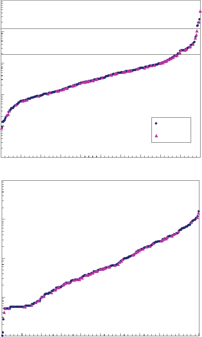
Figure 6. Frequency distribution of total mercury concentrations in fish, 1998–
2005, showing the percentage of samples that equalled or exceeded benchmark
or guideline concentrations. [USEPA methylmercury criterion for human health
(U.S. Environmental Protection Agency, 2001) = 0.3 µg/g wet weight; concern
level for piscivorous mammals (Yeardley and others, 1998) = 0.1 µg/g wet weight.]
Distributions of length-normalized THg concentrations
for the top four sh species collected (largemouth bass,
smallmouth bass, rainbow-cutthroat trout, and brown trout)
are each shown separately on U.S. maps in gures 7 through
10. Largemouth bass were collected across the broadest area
of all sh species but were mostly in eastern and southern
U.S. streams (g. 7). The highest length-normalized THg
concentrations in largemouth bass were found in coastal
streams in unmined basins of Louisiana, Georgia, Florida,
and North and South Carolina; one stream in a mined basin
from California was in this group of highest sh THg, but
concentrations at this site were lower than at most of the
coastal unmined sites in the group. In contrast, smallmouth
bass were not collected in the southern part of the United
States but instead were commonly collected in the upper
Midwest and northeastern United States (g. 8); the highest
length-normalized THg concentrations were at western sites
in mined basins, but also from the Hudson River in New York.
Rainbow and cutthroat trout were collected only in western
States and were the primary target top-predator sh for sites
in Oregon and Washington (g. 9). Because of their similar
habitats, feeding habits, and ability to hybridize where their
ranges overlap, these two species were combined for purposes
of data analysis. The highest length-normalized THg values in
rainbow-cutthroat trout were found at stream sites in mined,
urban, and geothermally affected basins in tributaries to the
Willamette Basin in western Oregon, and in North Creek near
Bothell, Wash., an urban site on a tributary to Puget Sound.
Brown trout were collected in isolated areas across the United
States, and the highest length-normalized THg concentrations
for this sh species were at several sites in mined basins of
Colorado and Nevada and in three unmined, undeveloped
basins of southern California, Colorado, and New York
(g. 10).

Spatial Distribution of Mercury in Fish, Bed Sediment, and Stream Water 15
11-7093_fig 07
0
250 500
MILES
0
250 500
KILOMETERS
0 100 200 MILES
0 100 200 KILOMETERS
0 500 1,000 MILES
0 500 1,000 KILOMETERS
0 50 100 MILES
0 50 100
KILOMETERS
EXPLANATION
MinedUnmined
Length-normalized total mercury,
wet-weight basis, largemouth bass,
as percentiles
Less than 25%
25 to 49%
50 to 74%
75 to 89%
Greater than or
equal to 90%
100°
90°
80°
70°
110°
120°
30°
40°
40°
30°
75°
70°
45°
40°
155°160°
22°
19°
70°
130°150°170°170°E
50°
60°
150° 140° 130°160°170°180°
50°
60°
70°
Figure 7. Spatial distribution of length-normalized total mercury concentrations in largemouth bass, 1998–2005.

16 Mercury in Fish, Bed Sediment, and Water from Streams Across the United States, 1998–2005
11-7093_fig 08
0
250 500
MILES
0
250 500
KILOMETERS
0 100 200 MILES
0 100 200 KILOMETERS
0 500 1,000 MILES
0 500 1,000 KILOMETERS
0 50 100 MILES
0 50 100
KILOMETERS
EXPLANATION
MinedUnmined
Length-normalized total mercury,
wet-weight basis, smallmouth bass,
as percentiles
Less than 25%
25 to 49%
50 to 74%
75 to 89%
Greater than or
equal to 90%
100°
90°
80°
70°
110°
120°
30°
40°
40°
30°
75°
70°
45°
40°
155°160°
22°
19°
70°
130°150°170°170°E
50°
60°
150° 140° 130°160°170°180°
50°
60°
70°
Figure 8. Spatial distribution of length-normalized total mercury concentrations in smallmouth bass, 1998–2005.

Spatial Distribution of Mercury in Fish, Bed Sediment, and Stream Water 17
11-7093_fig 09
0
250 500
MILES
0
250 500
KILOMETERS
0 100 200 MILES
0 100 200 KILOMETERS
0 500 1,000 MILES
0 500 1,000 KILOMETERS
EXPLANATION
MinedUnmined
Length-normalized total mercury,
wet-weight basis, rainbow-cutthroat
trout, as percentiles
Less than 25%
25 to 49%
50 to 74%
75 to 89%
Greater than or
equal to 90%
100°
90°
80°
70°
110°
120°
30°
40°
40°
30°
155°160°
22°
19°
70°
130°150°170°170°E
50°
60°
150° 140° 130°160°170°180°
50°
60°
70°
Figure 9. Spatial distribution of length-normalized total mercury concentrations in rainbow-cutthroat trout, 1998–2005.

18 Mercury in Fish, Bed Sediment, and Water from Streams Across the United States, 1998–2005
11-7093_fig 10
0
250 500
MILES
0
250 500
KILOMETERS
0 100 200 MILES
0 100 200 KILOMETERS
0 500 1,000 MILES
0 500 1,000 KILOMETERS
EXPLANATION
MinedUnmined
Length-normalized total mercury,
wet-weight basis, brown trout,
as percentiles
Less than 25%
25 - 49%
50 - 74%
75 - 89%
Greater than or
equal to 90%
100°
90°
80°
70°
110°
120°
30°
40°
40°
30°
155°160°
22°
19°
70°
130°150°170°170°E
50°
60°
150° 140° 130°160°170°180°
50°
60°
70°
Figure 10. Spatial distribution for percentiles of length-normalized total mercury concentrations in brown trout, 1998–2005.

Spatial Distribution of Mercury in Fish, Bed Sediment, and Stream Water 19
Bed Sediment
With the exception of sites in mined basins, many high
THg concentrations in bed sediment were in the northeast;
however, values in the top quartile of THg concentrations were
scattered across the United States (g. 11). Concentrations of
THg in bed sediment (dry-weight basis) ranged from 0.84 to
4,520 ng/g (table 3B). Concentrations were less than about 80
ng/g THg at 75 percent of sites and less than about 250 ng/g at
90 percent of sites (g. 12A).
Table 3B. Summary statistics for mercury in U.S. streams, 1998–2005: Total and methylmercury and ancillary chemical characteristics
of bed sediment.
[Mercury concentrations are on a dry-weight basis. Abbreviations: ng/g, nanograms per gram; µg/g, micrograms per gram; n, number of samples]
Parameter Site grouping Mean Median Std Dev Minimum Maximum n Units Comparison
Methylmercury
All sites 1.65 0.510 2.54 0.01 15.6 344 ng/g
No signicant
difference
Sites in unmined basins 1.73 0.510 2.62 0.01 15.6 257
Sites in mined basins 1.41 0.516 2.28 0.04 14.6 87
Total mercury
All sites 110 31.8 343 0.84 4,520 345 ng/g
Mined > Unmined
(p<0.01)
Sites in unmined basins 88.7 30.3 243 0.90 2,480 259
Sites in mined basins 175 48.5 539 0.84 4,520 86
Methyl/Total mercury
All sites 3.24 1.60 4.68 0.020 41.0 337 Percent
Unmined > Mined
(p<0.05)
Sites in unmined basins 3.26 1.72 4.58 0.020 41.0 253
Sites in mined basins 3.18 1.27 5.01 0.024 24.8 84
Loss-on-ignition
(LOI)
All sites 7.38 4.26 8.14 0.11 43.5 327 Percent
No signicant
difference
Sites in unmined basins 8.12 4.50 8.78 0.11 43.5 254
Sites in mined basins 4.78 3.51 4.52 0.50 27.7 73
Methylmercury/LOI
All sites 0.227 0.137 0.300 0.0040 2.56 325 (ng/g)/
percent
Mined > Unmined
(p<0.001)
Sites in unmined basins 0.195 0.125 0.255 0.0040 2.56 252
Sites in mined basins 0.338 0.201 0.402 0.0116 1.83 73
Total mercury/LOI
All sites 25.3 6.61 129 0.15 1,940 325 (ng/g)/
percent
Mined > Unmined
(p<0.0001)
Sites in unmined basins 10.1 5.91 14.5 0.15 122 253
Sites in mined basins 78.6 10.5 267 <0.58 1,940 72
Acid-volatile sulde
All sites 84.9 5.34 235 <0.01 2,630 252 µg/g
No signicant
difference
Sites in unmined basins 89.9 5.03 258 <0.01 2,630 187
Sites in mined basins 70.4 6.58 149 0.01 690 65
Concentrations of MeHg in bed sediment ranged from
0.01 to 15.6 ng/g (table 3B). The highest MeHg values were
from a group of New England coastal streams, including
sites in mined as well as unmined basins (g. 13). Some of
these New England streams, such as the Sudbury River in
Massachusetts, are unmined but known to have historical
industrial contamination of Hg in the basin (Massachusetts
Department of Environmental Protection, 1995; Flannagan
and others, 1999; Waldron and others, 2000; Wiener and
Shields, 2000; Chalmers, 2002). About 75 percent of all MeHg
values were less than 2 ng/g, and 90 percent of concentrations
were less than about 5 ng/g (g.12B).

20 Mercury in Fish, Bed Sediment, and Water from Streams Across the United States, 1998–2005
11-7093_fig 11
0
250 500
MILES
0
250 500
KILOMETERS
0 100 200 MILES
0 100 200 KILOMETERS
0 500 1,000 MILES
0 500 1,000 KILOMETERS
0 50 100 MILES
0 50 100
KILOMETERS
EXPLANATION
MinedUnmined
0.84 to 11.1
11.2 to 31.7
31.8 to 81.6
81.7 to 231
Total mercury, bed sediment, in
nanograms per gram dry weight
232 to 4520
100°
90°
80°
70°
110°
120°
30°
40°
40°
30°
75°
70°
45°
40°
155°160°
22°
19°
70°
130°150°170°170°E
50°
60°
150° 140° 130°160°170°180°
50°
60°
70°
Figure 11. Spatial distribution of total mercury concentrations in bed sediment, 1998–2005. [Percentiles shown: 0 to 24 (white), 25 to 49 (yellow), 50 to 74 (orange),
75 to 89 (red), and greater than or equal to 90 (purple).]
Spatial Distribution of Mercury in Fish, Bed Sediment, and Stream Water 21
11-7093-c_fig 12
A
B
0.10
1.00
10.00
100.00
1000.00
10000.00
0102030405060708090100
Unmined
Mined
Probable effect concentration = 1,060 ng/g
Threshold effect concentration = 180 ng/g
TOTAL MERCURY IN BED SEDIMENT,
IN NANOGRAMS PER GRAM DRY WEIGHT
0.01
0.10
1.00
10.00
100.00
0102030405060708090100
METHYLMERCURY IN BED SEDIMENT,
IN NANOGRAMS PER GRAM DRY WEIGHT
EXCEEDANCE FREQUENCY, IN PERCENT
Figure 12. Frequency distribution of mercury concentrations in bed sediment,
1998–2005, showing the percentage of samples that equalled or exceeded benchmark
or guideline concentrations; A, Total mercury; B, Methylmercury. [Probable Effect
Concentration, consensus-based (MacDonald and others, 2000) = 1,060 ng/g, dry weight;
Threshold Effect Concentration, consensus-based (MacDonald and others, 2000) = 180
ng/g dry weight.]

22 Mercury in Fish, Bed Sediment, and Water from Streams Across the United States, 1998–2005
11-7093_fig 13
0.01 to 0.13
0.14 to 0.50
0.51 to 2.02
2.03 to 5.03
Methylmercury, bed sediment,
in nanograms per gram dry weight
5.04 to 15.6
0
250 500
MILES
0
250 500
KILOMETERS
0 100 200 MILES
0 100 200 KILOMETERS
0 500 1,000 MILES
0 500 1,000 KILOMETERS
0 50 100 MILES
0 50 100
KILOMETERS
EXPLANATION
MinedUnmined
100°
90°
80°
70°
110°
120°
30°
40°
40°
30°
75°
70°
45°
40°
155°160°
22°
19°
70°
130°150°170°170°E
50°
60°
150° 140° 130°160°170°180°
50°
60°
70°
Figure 13. Spatial distribution of methylmercury concentrations in bed sediment, 1998–2005. [Percentiles shown: 0 to 24 (white), 25 to 49 (yellow),
50 to 74 (orange), 75 to 89 (red), and greater than or equal to 90 (purple).]

Spatial Distribution of Mercury in Fish, Bed Sediment, and Stream Water 23
Table 3C. Summary statistics for mercury in U.S. streams, 1998–2005: Total and methylmercury and ancillary water quality
characteristics of unfiltered stream water.
[Values equal to 1/2 minimum reporting limits were substituted for censored values in computations. Abbreviations: DOC, dissolved organic carbon; UV,
ultraviolet absorbance at 254 nm; SUVA, specic UV absorbance at 254 nm; nm, nanometers; (L/mg C)/m, liters per milligram carbon per meter; ng/L,
nanograms per liter; mg/L, milligrams per liter; µS/cm, microsiemens per centimeter at 25 degrees Celsius; n, number of samples]
Parameter Site grouping Mean Median Std Dev Min Max n Units Comparison
Methylmercury
All sites 0.19 0.11 0.35 <0.010 4.11 337 ng/L
No signicant
difference
Sites in unmined basins 0.20 0.11 0.37 <0.010 4.11 257
Sites in mined basins 0.18 0.10 0.31 <0.010 2.02 80
Total mercury
All sites 8.22 2.09 32.8 0.27 446 336 ng/L
Mined > Unmined
(p<0.0001)
Sites in unmined basins 2.96 1.90 5.29 0.27 75.1 250
Sites in mined basins 23.5 3.79 62.1 0.48 446 86
Methyl/Total mercury
All sites 7.08 4.60 8.18 0.02 81.5 328 Percent
Unmined > Mined
(p<0.0001)
Sites in unmined basins 7.46 5.35 6.72 0.19 46.8 249
Sites in mined basins 5.87 2.37 11.6 0.02 81.5 79
Specic conductance All sites 389 247 493 15.6 6,080 349 µS/cm Mined > Unmined
(p<0.001)
Sites in unmined basins 349 246 467 15.6 6,080 263
Sites in mined basins 513 252 551 34.1 2,350 86
pH All sites 7.48 7.50 0.73 3.30 10.1 352 Standard units Mined > Unmined
(p<0.01)
Sites in unmined basins 7.38 7.42 0.72 5.50 10.1 264
Sites in mined basins 7.78 7.90 0.70 3.30 9.00 88
Suspended sediment All sites 75.4 7.00 501 0 6,170 177 mg/L No signicant
difference
Sites in unmined basins 26.3 7.00 53.1 0 391 130
Sites in mined basins 212 8.00 966 1 6,170 47
DOC All sites 5.09 3.80 6.49 0.34 76.9 349 mg/L Unmined > Mined
(p<0.0001)
Sites in unmined basins 5.82 4.38 7.29 0.34 76.9 261
Sites in mined basins 2.90 2.61 1.77 0.40 11.6 88
UV All sites 0.15 0.11 0.17 0.003 1.2 138 Dimensionless
Unmined > Mined
(p<0.001)
Sites in unmined basins 0.18 0.13 0.18 0.005 1.2 107
Sites in mined basins 0.08 0.07 0.05 0.003 0.3 31
SUVA All sites 2.92 2.80 1.43 0.30 15.5 138 (L/mg C)/m No signicant
difference
Sites in unmined basins 2.92 2.90 0.91 0.60 5.7 107
Sites in mined basins 2.92 2.60 2.52 0.30 15.5 31
Sulfate All sites 45.9 10.9 123 0.09 954 343 mg/L Mined > Unmined
(p<0.01)
Sites in unmined basins 28.3 9.95 73.7 0.09 954 263
Sites in mined basins 104 16.1 208 0.47 860 80
Stream Water
There was wide variation in concentrations of THg
in unltered water across the United States, as one might
expect for a dataset that included sites that were relatively
pristine to sites in gold- or Hg-mined basins (table 3C;
g. 14). Concentrations of unltered THg ranged from 0.27
to 446 ng/L, and the median value was 2.09 ng/L. THg
concentrations were less than about 4 ng/L at 75 percent
of sites and less than about 9 ng/L at 90 percent of sites
(g. 15A).
Concentrations of MeHg in unltered water were
somewhat less variable than for THg across sites (g. 16).
Values ranged from less than 0.01 to 4.11 ng/L, and the
median MeHg concentration was 0.11 (table 3C). MeHg
concentrations were less than about 0.2 ng/L at 75 percent of
the sites and less than about 0.4 ng/L at 90 percent of sites
(g. 15B). Moreover, MeHg concentrations at 97 percent of
the sites were less than 0.8 ng/L, which is consistent with
ndings of Krabbenhoft and others (2007), who reviewed
the literature and found that most surface waters had MeHg
concentrations in the range of approximately 0.04 to 0.8 ng/L
(St. Louis and others, 1994; Hurley and others, 1995; Babiarz
and others, 1998; Bodaly and others, 1998; Gilmour and
others, 1998; Krabbenhoft and others, 1999).

24 Mercury in Fish, Bed Sediment, and Water from Streams Across the United States, 1998–2005
11-7093_fig 14
0
250 500
MILES
0
250 500
KILOMETERS
0 100 200 MILES
0 100 200 KILOMETERS
0 500 1,000 MILES
0 500 1,000 KILOMETERS
0 50 100 MILES
0 50 100
KILOMETERS
EXPLANATION
MinedUnmined
Total mercury, unfiltered water,
in nanograms per liter
0.27 to 1.30
1.31 to 2.08
2.09 to 3.88
3.89 to 9.00
9.01 to 446
100°
90°
80°
70°
110°
120°
30°
40°
40°
30°
75°
70°
45°
40°
155°160°
22°
19°
70°
130°150°170°170°E
50°
60°
150° 140° 130°160°170°180°
50°
60°
70°
Figure 14. Spatial distribution of total mercury concentrations in unfiltered stream water,1998–2005. [Percentiles shown: 0 to 24 (white),
25 to 49 (yellow), 50 to 74 (orange), 75 to 89 (red), and greater than or equal to 90 (purple).]

Spatial Distribution of Mercury in Fish, Bed Sediment, and Stream Water 25
Figure 15. Frequency distribution of mercury concentrations in unfiltered water, 1998–2005,
showing the percentage of samples that equalled or exceeded benchmark or guideline
concentrations; A, Total mercury; B, Methylmercury. [Great Lakes States 30-day standard for fish-
eating wildlife (U.S. Environmental Protection Agency,1997) = 1.3 ng/L.]
11-7093-c_fig 15
TOTAL MERCURY IN UNFILTERED WATER,
IN NANOGRAMS PER LITER
METHYMERCURY IN UNFILTERED WATER,
IN NANOGRAMS PER LITER
EXCEEDANCE FREQUENCY, IN PERCENT
A
B
0.10
1.00
10.00
100.00
1,000.00
0102030405060708090100
Unmined
Mined
30-day standard for fish-eating wildlife = 1.3 ng/L
0.001
0.010
0.100
1.000
10.000
0102030405060708090100

26 Mercury in Fish, Bed Sediment, and Water from Streams Across the United States, 1998–2005
11-7093_fig 16
0
250 500
MILES
0
250 500
KILOMETERS
0 100 200 MILES
0 100 200 KILOMETERS
0 500 1,000 MILES
0 500 1,000 KILOMETERS
0 50 100 MILES
0 50 100
KILOMETERS
EXPLANATION
MinedUnmined
Methylmercury, unfiltered water,
in nanograms per liter
< 0.010 to 0.043
0.044 to 0.106
0.107 to 0.193
0.194 to 0.395
0.396 to 4.11
100°
90°
80°
70°
110°
120°
30°
40°
40°
30°
75°
70°
45°
40°
155°160°
22°
19°
70°
130°150°170°170°E
50°
60°
150° 140° 130°160°170°180°
50°
60°
70°
Figure 16. Spatial distribution of methylmercury concentrations in unfiltered stream water, 1998–2005. [Percentiles shown: 0 to 24 (white), 25 to 49 (yellow),
50 to 74 (orange), 75 to 89 (red), and greater than or equal to 90 (purple).]

Comparisons Among Fish, Bed Sediment, and Stream Water 27
Comparisons to Benchmarks and
Guidelines
Hg concentrations in sh at most sites (71 percent, 208 of
291 sites) exceeded the value of 0.1 µg/g THg (ww) that is of
concern for the protection of sh-eating mammals, including
mink and otters (g. 6; Yeardley and others, 1998; Peterson
and others, 2007). Concentrations at 27 percent of the sites
(79 of 291) exceeded 0.3 μg/g THg ww in sh. As mentioned
earlier, most of the Hg found in sh tissue is MeHg (Huckabee
and others, 1979; Grieb and others, 1990; Bloom 1992), and
a concentration of 0.3 µg/g MeHg ww in sh is the USEPA
MeHg criterion for the protection of human health (U.S.
Environmental Protection Agency, 2001, 2009).
Two sediment-quality guidelines were used to evaluate
THg concentrations in bed sediment in our study. These
consensus-based concentrations of MacDonald and others
(2000) are currently considered to be the best predictive
guidelines. However, MacDonald and others (2000) noted
that the consensus-based Threshold Effect Concentration
(TEC) for THg correctly predicted toxicity only 34 percent
of the time, whereas the consensus-based Probable Effect
Concentration (PEC) correctly predicted toxicity 100 percent
of the time although based on only 4 values. Because the
primary toxic form of Hg is MeHg, THg-based toxicity
estimates are not expected to be highly accurate; however,
MeHg-based guidelines are unavailable at this time. In our
study, concentrations of THg at 12 percent of sites (40 of 345
sites) exceeded the TEC of 180 ng/g. Total Hg in bed sediment
from six of the sites exceeded the PEC of 1,060 ng/g; these
sites included two western sites in mined basins (South
Fork Coeur d’Alene River and Carson River below Carson
Diversion Dam) and four sites from the northeast (Mousam
River in Maine; Aberjona, Assabet, and Neponset Rivers near
Boston, Massachussetts). These results indicate the potential
for toxic effects on benthic communities at some sites sampled
as part of this study.
Because of the complicated nature of Hg methylation and
bioaccumulation, there are currently no national guidelines
for protection of wildlife from exposure to Hg in water.
However, of 336 sites with data for THg in unltered water,
THg at three-quarters of the sites exceeded 1.3 ng/L, the
30-day standard derived by the USEPA for Great Lakes
States sh-eating wildlife and slightly less than the value of
1.8 ng/L derived for protection of eagles (U.S. Environmental
Protection Agency, 1995a, 1995b, 1997; Wolfe and others,
2007). Concentrations of unltered THg at 14 sites exceeded
26 ng/L, the Interim Canadian Water Quality Guideline for the
protection of freshwater life (Environment Canada, 2005). All
but one site with unltered THg concentrations greater than
26 ng/L were in the western United States, in basins where
gold and (or) Hg mining took place in the past. The exception,
Whitewood Creek above Lead, S.D., was within the highly
mineralized area of the Black Hills of South Dakota (Norton,
1975; Goddard, 1988). There are gold mines in the area that
could have contributed to high Hg concentrations, but some
sites in this geochemically rich region are likely to be naturally
enriched in Hg. The unltered THg concentration above Lead
was similar to that found downstream at Deadwood (75.1 and
77.8 ng/L, respectively). In contrast to the sampling timing for
the majority of our synoptic sites, the South Dakota sampling
was intentionally timed to catch runoff with high-suspended
sediment loads, when most of the Hg was in the particulate
phase (Steve Sando, U.S. Geological Survey, oral commun.,
October 2007).
Comparisons Among Fish, Bed
Sediment, and Stream Water
Because of bioaccumulation and biomagnication, Hg
concentrations in sh were several orders of magnitude higher
than in stream water. Overall, results of our study agreed
with results in the literature for lakes and other waterbody
types that have described relatively large differences in
mean concentrations among sh, bed sediment, and water
(Wiener and Stokes, 1990; Wiener, 1995; U.S. Environmental
Protection Agency, 1997; Mason and others, 2000). We found
a high accumulation of Hg in top-predator sh compared to
stream water and bed sediment. This accumulation resulted in
Hg concentrations in top-predator sh that were more than six
orders of magnitude higher than concentrations of Hg in the
water that the sh inhabit (g. 17).
For all sh species and sites combined, the mean Biota
Accumulation Factor (BAF, in log
10
; see equation 1, p. 8) for
THg in sh relative to MeHg in water was 6.33 L/kg (range
= 4.36 to 7.59) and for THg in sh relative to MeHg in bed
sediment was 3.42 (range = 1.52 to 5.09) (table 4A). The
BAF values determined in our studies were not signicantly
different at sites in mined basins when compared to sites in
unmined basins. However, mean and median BAF values
were lower for bed sediment than for water (tables 4B and
4C). Our mean water BAF value of 6.33 L/kg was slightly
lower than the national mean BAF value of 6.40 L/kg reported
by the USEPA for Hg in riverine sh relative to water (U.S.
Environmental Protection Agency, 2000).

28 Mercury in Fish, Bed Sediment, and Water from Streams Across the United States, 1998–2005
11-7093-c Mercury SIR_fig 17
x
x
x
x
x
x
(337)
Number of values
EXPLANATION
Methylmercury,
in unfiltered
water
Methylmercury,
in bed
sediment (dw)
Total mercury,
in fish (ww)
10
-9
10
1
10
-1
10
-3
10
-5
10
-7
MERCURY CONCENTRATION, IN PARTS PER MILLION
(337)
(344)
(291)
VERTICAL LINES —Lines from
rectangle extend to the last data
point that is < 1.5 times the
semiquartile range
75th PERCENTILE
MEDIAN
25th PERCENTILE
SEMIQUARTILE
RANGE
x
o
OUTSIDE VALUE—Values are more
than 1.5 times the semiquartile
range from the top or bottom of the
rectangle
FAR OUT VALUE—Values are more than
3.0 times the semiquartile range from
the top or bottom of the rectangle
Figure 17. Statistical distributions of mercury concentrations in fish, bed sediment, and water, 1998–2005. (dw, dry
weight; ww, wet weight)
Table 4A.
Summary statistics for mercury Biota Accumulation Factors (BAFs) for fish from U.S. streams, 1998–2005: BAFs for fish with
respect to water and bed sediment, all species.
[Abbreviations: BAF, Biota Accumulation Factor; water BAF values are for THg in sh with respect to MeHg in ltered water, in log
10
(liters per kilogram);
sediment BAF values are for THg in sh with respect to MeHg in bed sediment, in log
10
(grams per gram); Std Dev, standard deviation; n, number of samples]
Parameter Site grouping Mean Median Std Dev Minimum Maximum n
BAF (water)
All sites 6.33 6.33 0.50 4.36 7.59 166
Sites in unmined basins 6.32 6.30 0.50 4.36 7.59 128
Sites in mined basins 6.36 6.35 0.48 5.46 7.47 38
BAF (sediment)
All sites 3.42 3.43 0.76 1.52 5.09 229
Sites in unmined basins 3.45 3.43 0.80 1.52 5.09 175
Sites in mined basins 3.32 3.49 0.61 1.92 4.42 54

Comparisons to Benchmarks and Guidelines 29
Table 4B. Summary statistics for mercury Biota Accumulation Factors (BAFs) for fish from U.S. streams, 1998–2005: BAFs for fish with
respect to water, individual species.
[Abbreviations: BAF, Biota Accumulation Factor; water BAF values are for THg in sh with respect to MeHg in ltered water, in log
10
(liters per kilogram);
Std Dev, standard deviation; ND, no data; *, insufcient data to compute summary metric; n, number of samples]
Parameter Site grouping Mean Median Std Dev Minimum Maximum n
Largemouth bass All sites 6.61 6.61 0.46 5.22 7.59 38
Sites in unmined basins 6.58 6.60 0.47 5.22 7.59 33
Sites in mined basins 6.82 6.81 0.38 6.34 7.39 5
Smallmouth bass All sites 6.32 6.37 0.48 5.25 7.08 20
Sites in unmined basins 6.41 6.38 0.43 5.25 7.08 15
Sites in mined basins 6.02 5.93 0.53 5.46 6.70 5
Rock bass All sites 6.18 6.24 0.42 5.38 7.00 11
Sites in unmined basins 6.18 6.24 0.42 5.38 7.00 11
Sites in mined basins ND ND ND ND ND ND
Spotted bass All sites 6.59 6.52 0.35 6.09 7.32 12
Sites in unmined basins 6.52 6.40 0.38 6.09 7.32 8
Sites in mined basins 6.73 6.72 0.27 6.42 7.07 4
Pumpkinseed All sites ND ND ND ND ND ND
Sites in unmined basins ND ND ND ND ND ND
Sites in mined basins ND ND ND ND ND ND
Rainbow-cutthroat trout
All sites 6.31 6.27 0.40 5.54 7.47 26
Sites in unmined basins 6.26 6.29 0.36 5.54 6.92 19
Sites in mined basins 6.43 6.26 0.51 5.92 7.47 7
Brown trout All sites 6.04 6.04 0.42 5.25 6.96 18
Sites in unmined basins 5.87 6.03 0.34 5.25 6.25 9
Sites in mined basins 6.21 6.34 0.44 5.63 6.96 9
Channel catsh All sites 6.12 6.02 0.36 5.56 6.76 11
Sites in unmined basins 6.08 6.00 0.36 5.56 6.76 9
Sites in mined basins * * * 5.84 6.02 2

30 Mercury in Fish, Bed Sediment, and Water from Streams Across the United States, 1998–2005
Table 4C. Summary statistics for mercury Biota Accumulation Factors (BAFs) for fish from U.S. streams, 1998–2005: BAFs for fish with
respect to bed sediment, individual species.
[Abbreviations: BAF, Biota Accumulation Factor; sediment BAF values are for THg in sh with respect to MeHg in bed sediment, in log
10
(grams per gram);
Std Dev, standard deviation; ND, no data, *, insufcient data to compute summary metric; n, number of samples]
Parameter Site grouping Mean Median Std Dev Minimum Maximum n
Largemouth bass All sites 3.99 4.08 0.67 2.37 5.09 51
Sites in unmined basins 4.08 4.26 0.71 2.37 5.09 42
Sites in mined basins 3.59 3.57 0.23 3.12 3.91 9
Smallmouth bass All sites 3.43 3.55 0.63 1.73 4.96 44
Sites in unmined basins 3.41 3.40 0.65 1.73 4.96 36
Sites in mined basins 3.50 3.72 0.52 2.39 3.87 8
Rock bass All sites 3.24 3.20 0.71 2.09 4.61 14
Sites in unmined basins 3.24 3.20 0.71 2.09 4.61 14
Sites in mined basins ND ND ND ND ND ND
Spotted bass All sites 4.07 4.07 0.35 3.53 4.51 14
Sites in unmined basins 4.23 4.37 0.32 3.53 4.51 9
Sites in mined basins 3.76 3.78 0.14 3.54 3.90 5
Pumpkinseed All sites 1.91 2.04 0.26 1.52 2.16 5
Sites in unmined basins 1.91 2.04 0.26 1.52 2.16 5
Sites in mined basins ND ND ND ND ND ND
Rainbow-cutthroat trout All sites 3.16 3.13 0.51 2.20 4.10 26
Sites in unmined basins 3.18 3.15 0.47 2.20 3.98 19
Sites in mined basins 3.12 2.93 0.66 2.35 4.10 7
Brown trout All sites 3.03 2.97 0.63 1.92 4.25 17
Sites in unmined basins 3.01 2.75 0.52 2.51 3.82 8
Sites in mined basins 3.04 3.04 0.75 1.92 4.25 9
Channel catsh All sites 2.89 2.75 0.46 2.38 3.67 11
Sites in unmined basins 2.90 2.75 0.46 2.38 3.67 9
Sites in mined basins * * * 2.38 3.32 2
Comparisons Between Mined and
Unmined Basins
All sites in Hg-mined basins and most sites in gold-
mined basins were in the western half of the United States
(g. 3). Across all sites, sh Hg, as wet weight (raw or length-
normalized), was not signicantly different between sites in
unmined basins and mined basins, except for smallmouth bass.
That exception was solely due to a single high outlier for the
composite sample of smallmouth bass from the Carson River
at Dayton, Nev., a mined basin. Concentrations of MeHg
in bed sediment and unltered stream water from sites in
unmined basins were not signicantly different from those in
mined basins; however, THg concentrations were signicantly
higher in bed sediment and stream water from sites in mined
basins (tables 3B,C; g.18).
It also should be noted that the percentages of MeHg
(percent MeHg/THg) in bed sediment and unltered water
were signicantly higher in unmined basins (tables 3B, 3C).
The percentage of MeHg is considered to be a useful
estimate of methylation efciency (Gilmour and others,
1998). Although THg concentrations in unltered water
were higher as a group from streams in mined basins, MeHg
concentrations from many of these same streams were not
high relative to those at other sampled sites. More importantly,
water from many sites in unmined basins with relatively low
THg was relatively high in MeHg. This nding emphasizes the
importance of Hg methylation in these ecosystems.
Examination of Hg relations to environmental
characteristics for sh species from sites in mined basins
was limited to largemouth bass and brown trout because of
small sample sizes for other species. Concentrations of Hg
in largemouth bass at these sites increased with increasing
suspended sediment (r
s
= 0.98, p < 0.05, n = 5) and THg in
unltered water (r
s
= 0.67, p < 0.05, n = 9). In contrast, Hg
in brown trout at sites in mined basins increased signicantly
with increasing MeHg concentration in unltered water
(r
s
= 0.93, p < 0.01, n = 7).

Comparisons Between Mined and Unmined Basins 31
11-7093-c_fig 18
x
x
x
x
x
x
x
(86) (259) (87) (257)
MERCURY CONCENTRATION IN BED SEDIMENT,
IN NANOGRAMS PER GRAM
10
-2
10
-1
10
0
10
1
10
2
10
3
10
4
Bed Sediment
Unfiltered Water
x
x
x
x
x
x
x
o
x
x
x
x
x
x
(86) (250) (80) (257)
Total mercury Total mercury Methylmercury Methylmercury
MERCURY CONCENTRATION IN UNFILTERED WATER,
IN NANOGRAMS PER LITER
10
-3
10
-2
10
-1
10
0
10
1
10
2
10
3
Unmined
Mined
Total mercury Total mercury Methylmercury Methylmercury
(86)
Number of values
EXPLANATION
VERTICAL LINES —Lines from
rectangle extend to the last data
point that is < 1.5 times the
semiquartile range
75th PERCENTILE
MEDIAN
25th PERCENTILE
SEMIQUARTILE
RANGE
x
o
OUTSIDE VALUE—Values are more
than 1.5 times the semiquartile
range from the top or bottom of the
rectangle
FAR OUT VALUE—Values are more than
3.0 times the semiquartile range from
the top or bottom of the rectangle
Figure 18. Statistical distributions of mercury concentrations in bed sediment and unfiltered water at stream
sites in mined and unmined basins, 1998–2005.

32 Mercury in Fish, Bed Sediment, and Water from Streams Across the United States, 1998–2005
Factors Related to Mercury
Bioaccumulation in Fish
The remainder of this report describes relations between
environmental characteristics and length-normalized Hg
concentrations (micrograms per gram per meter) in unmined
basins for the sh species that were most commonly collected:
largemouth bass, smallmouth bass, rainbow-cutthroat
trout, brown trout, pumpkinseed, rock bass, spotted bass,
and channel catsh. Data for sites in mined basins were
removed from these analyses to allow for evaluation of
factors other than mining that could be important in sh Hg
bioaccumulation. Most of the 89 sites in mined basins were
in just two LULC categories: undeveloped (61 sites) or mixed
(21 sites), and for several sh species—especially brown
trout—the land-use relation often became weak or nonexistent
when sites in mined basins were included.
Comparisons Among Land-Use/Land-Cover
Categories
Signicant differences among LULC categories were
found for unmined basins (but not for mined basins) with
respect to Hg. For unmined sites, largemouth bass from
predominantly undeveloped or mixed-land-use basins were
signicantly higher in Hg than those from urban basins and
were somewhat higher (p = 0.059) than those from agricultural
basins (g. 19); a similar difference was seen between
undeveloped and urban basins for brown trout. Spotted bass
from undeveloped basins were somewhat higher in Hg than
those from agricultural basins (p = 0.051). In contrast to sh
THg, bed sediment THg (whether normalized by LOI or not)
and AVS were higher at urban sites compared to agricultural,
undeveloped, or mixed-land-use sites. Although there were no
signicant differences among LULC categories for MeHg in
bed sediment, the percentage of MeHg in bed sediment was
higher at undeveloped sites than at urban sites. Undeveloped
sites tended to have more wetland and forest cover in the
basin. Differences among LULC categories were not found for
THg or MeHg in unltered water.
11-7093-c_fig 19
TOTAL MERCURY IN LARGEMOUTH BASS, IN MICROGRAMS
PER GRAM PER METER,
WET-WEIGHT BASIS
(8) (11) (10) (22)
Agriculture Urban Undeveloped Mixed
(8)
Number of values
EXPLANATION
10
0
10
-1
10
1
VERTICAL LINES —Lines from
rectangle extend to the last data
point that is < 1.5 times the
semiquartile range
75th PERCENTILE
MEDIAN
25th PERCENTILE
SEMIQUARTILE
RANGE
Figure 19. Statistical distributions of length-normalized mercury concentrations in largemouth bass for U.S. streams
draining various land-use/land-cover categories, 1998–2005.

Factors Related to Mercury Bioaccumulation in Fish 33
For those sh species with enough data available to test
subcategories within the undeveloped LULC category for
unmined sites (largemouth bass, smallmouth bass, rock bass,
and brown trout), only largemouth bass showed signicant
differences between two subcategories: Hg concentrations
in largemouth bass from sites in forested areas with high
percentages of wetland (>15 percent) were signicantly
higher than in largemouth bass from sites in forested areas
with low percentages of wetland (<10 percent) (means ±
standard deviations were 2.92 ± 0.79 (µg/g)/m and 1.28 ±
0.05 (µg/g)/m, n = 6 and 3, respectively). The comparison
should be viewed with caution due to the small sample sizes.
Fish Species-Specific Relations with
Environmental Characteristics
Relations between sh Hg and environmental
characteristics varied in their signicance with the group of
sh examined (table 5). Fish length correlated positively with
Hg concentration for largemouth bass, rock bass, and rainbow-
cutthroat trout, so length-normalized Hg concentrations for all
sh were used in comparisons to environmental characteristics
(Boudou and Ribeyre, 1983; Ribeyre and Boudou, 1984;
Goldstein and others, 1996, Brumbaugh and others, 2001).
Perhaps because of differences in species spatial distribution,
as well as feeding habits, many statistically signicant
relations to environmental characteristics were found for Hg in
largemouth bass (n = 52, unmined), whereas none were found
for smallmouth bass (n = 51, unmined). Sample numbers
of other sh species were more limited (n < 20, unmined),
and signicant relations also were less common than for
largemouth bass. The apparent absence of relations for these
other sh species may have been due in part to small sample
sizes. Most bass samples in our study were from the eastern
and southern United States. Largemouth bass appeared to
be a good indicator for Hg in top-predator sh on the basis
of (1) its ability to accumulate Hg from a predominantly
piscivorous diet; (2) relations between Hg in largemouth bass
and LULC, and MeHg in water or bed sediment; and (3) its
generally ubiquitous distribution and status as a game sh.
Factors related to Hg bioaccumulation in largemouth bass
from unmined basins were subsequently examined in greater
detail.
Stepwise multiple-linear regression revealed that
increasing length-normalized Hg concentrations in largemouth
bass from unmined basins were primarily related to increasing
basin percentages of evergreen forest and woody wetland,
especially with increasing proximity of evergreen forest and
woody wetland to the sampling site (adjusted r
2
= 0.66):
LMB ef
ww
LMB
ln[Hg ] = -0.592 + 0.0319 arcsin [L ]
+ 0.0194 arcsin [L ] ,
where
Hg is the length-normalized THg concentration
in largemouth bass, in micrograms per gram
ef
ww
per meter,
L is the distance-weighted percentage of basin
LULC that is evergreen forest, and
L is the distance-weighted percentage of basin
LULC that is woody wetland.
(2)
This equation underscores the sensitivity of these two
LULC types in comparison to other types with regard to
Hg bioaccumulation in largemouth bass. Evergreen forest
and woody wetland were positively correlated with each
other (r
s
= 0.60) in the largemouth bass dataset even though
these characteristics were uncorrelated in the larger dataset.
Redundancy Analysis (RDA) conrmed the signicance
of these two characteristics and additionally indicated that
increasing amounts of MeHg in unltered stream water and
LOI normalized MeHg concentrations in bed sediment, and
decreasing pH and dissolved sulfate, were important for
explaining variability in sh-Hg concentrations (g. 20).
Normalizing MeHg in bed sediment by organic content (as
measured by LOI) provided a way to account for differences
in the Hg concentrations of bed sediment collected from zones
of inorganic sediment as compared to zones of organic muck.
The similar results from multiple regression and RDA conrm
the importance of evergreen forest, woody wetland, and
MeHg in bed sediment and stream water for predicting THg in
largemouth bass. Details of these relations are provided below.
The strength and direction of relations to LULC varied
with sh species examined. As mentioned above, as the
percentage of evergreen forest and woody wetland in the
basin increased, Hg concentrations in largemouth bass also
increased (gs. 21A, B). When the percentages of woody
wetland were distance-weighted, r
s
values for largemouth
bass increased from 0.62 to 0.72 (table 5). This indicates that
the closer woody wetland was to the sampling site, the higher
the concentration of sh Hg. Spotted bass and brown trout
Hg were also positively correlated with evergreen forest,
including distance-weighted evergreen forest (g. 21C, 21D).
Hg in smallmouth bass did not correlate signicantly with
either forest or wetland. In general, positive relations were
also seen between sh Hg and either total forest or total
wetland in the basin; however, the relations were weaker than
with evergreen forest or woody wetland.

34 Mercury in Fish, Bed Sediment, and Water from Streams Across the United States, 1998–2005
Table 5. Spearman rank correlation coefficients (r
s
) for relations between length-normalized total mercury
in composite samples of fish and selected environmental characteristics for U.S. streams, 1998–2005.
[Denitions of variable abbreviations are listed in Appendix 1. Values are for sites in unmined basins only. Color coding of r
s
based on p values, p < 0.001 (pink), p < 0.01 (orange), and p < 0.05 (yellow). Abbreviations: n, number of samples available for
correlation;*, insufcient n or too many values less than the detection limit]
Largemouth
bass
Smallmouth
bass
Rock bass
Spotted bass
Pumpkinseed
Rainbow -
cutthroat trout
Brown trout
Channel catfish
Maximum n 52 51 17 9 16 19 13 10
Streamwater
pH -0.43 -0.03 -0.14 0.24 0.30 0.18 -0.25 -0.49
DOC 0.13 0.01 -0.61 -0.45 0.04 0.28 -0.60 0.15
Sulfate -0.54 -0.23 -0.04 -0.52 -0.41 0.65 -0.65 0.18
UMeHg 0.50 0.19 -0.04 -0.07 0.79 0.24 -0.26 -0.12
UTHg 0.37 0.09 -0.24 -0.17 -0.52 0.54 -0.35 0.21
UMeHg/UTHg 0.36 0.21 -0.42 0.45 0.86 -0.38 -0.52 -0.19
Bed sediment
SMeHg 0.07 -0.01 0.13 0.47 0.67 0.41 0.31 -0.20
STHg -0.09 -0.08 0.35 -0.10 -0.17 0.32 -0.26 -0.08
SMeHg/STHg 0.32 0.04 -0.04 0.73 0.74 0.16 0.85 0.12
SMeHg/LOI 0.35 0.01 -0.03 0.60 0.29 0.56 0.42 -0.27
STHg/LOI -0.03 -0.05 0.07 -0.23 -0.59 0.40 -0.77 0.03
Land use/land cover, percentage of basin area
SUM_FOREST 0.56 0.25 0.05 0.68 0.19 * 0.62 0.47
EVR_FOREST 0.77 0.18
-0.25 0.72 0.44 * 0.82 0.39
EVR_FOREST_DW 0.77 0.16 -0.37 0.72 0.54 * 0.86 0.31
SUM_WETLAND 0.46 -0.19 -0.52 -0.12 0.25 0.15 -0.18 -0.21
WOODWETLAND 0.62 -0.28 -0.50 0.28 0.32 0.33 -0.19 -0.04
WOODWETLAND_DW 0.72 -0.25 -0.42 0.17 0.35 0.33 -0.25 -0.15
HERBWETLAND -0.01 -0.06 -0.51 -0.15 -0.14 -0.07 -0.38 -0.19
HERBWETLAND_DW 0.06 -0.03 -0.40 -0.15 -0.04 -0.06 -0.37 -0.13
SUM_UNDEVELOPED 0.58 0.22 -0.11 0.70 0.20 -0.60 0.67 0.31
SUM_URBAN -0.48 -0.20 0.13 -0.20 -0.16 * -0.58 0.25
POPDEN00 -0.50 -0.22 0.37 -0.60 -0.39 * -0.75 0.27
SUM_AGRICULTURE -0.14 -0.24 0.14 -0.72 0.24 * -0.78 -0.31
ROW_CROP 0.10 -0.31 0.05 -0.70 0.30 0.08 -0.65 -0.39
ROW_CROP_DW 0.11 -0.31 0.05 -0.70 0.22 * -0.66 -0.30
Other
AWET.PRE 0.28 -0.26 -0.01 0.53 -0.46 * -0.31 0.10
ATOT.SEI -0.16 0.02 0.76 * 0.09 -0.20 -0.32 0.12

Factors Related to Mercury Bioaccumulation in Fish 35
11-7093-c Mercury SIR_fig 20
-1.0 1.2
-1.0 1.0
Sulfate,
unfiltered water
Methylmercury,
unfiltered water
Methylmercury/Loss on ignition,
bed sediment
Woody wetland,
distance weighted
RDA Axis 2
RDA Axis 1
pH,
unfiltered water
Fish mercury, wet weight
Fish mercury/length, wet weight
Evergreen forest, distance weighted
Figure 20. Redundancy Analysis (RDA) showing relative importance of selected environmental characteristics (blue arrows and
labels) to concentrations of mercury in largemouth bass (green arrows and labels), 1998–2005. (Arrows extending in the same
direction indicate a positive correlation, arrows in opposite directions indicate a negative correlation, and arrows at right angles
indicate no correlation; arrow length indicates the relative importance of the variable in the relation.)
LULC data that correlated negatively with sh Hg
included the percentage of urban developed land and Census
2000 population density (g. 21E, largemouth bass; g 21F,
brown trout), and percentage of row crops (brown trout only;
table 5). Chalmers (2002) in the New England Coastal Basins
regional study data included here, also found a negative
correlation (r
s
= -0.72) between sh Hg and population
density. Brumbaugh and others (2001) found a negative
correlation with urban land and sh Hg, although most of
the sh sampled from urban streams were largemouth or
smallmouth bass. The above results underscore the importance
of considering LULC and especially its proximity to the
sampling site when interpreting sh-Hg concentrations.
Although sh Hg in largemouth bass, spotted bass,
pumpkinseed, brown trout, and rainbow-cutthroat trout
correlated with various measures of bed sediment Hg, sh
Hg in smallmouth bass, rock bass, and channel catsh did not
(table 5). Fish Hg correlated with LOI only for pumpkinseed
(r
s
= 0.58, p < 0.05), whereas Hg in largemouth bass, spotted
bass, and rainbow-cutthroat trout correlated positively with
bed sediment MeHg as normalized by LOI (g. 21G–21I),
and, in general, these correlations were higher than with
bed-sediment MeHg concentrations that were not normalized
by LOI (table 5). An exception was found for pumpkinseed;
sh Hg in pumpkinseed was more highly correlated with
bed-sediment MeHg concentrations not normalized by LOI
(g. 21J). An estimate of Hg methylation potential, the
percentage of MeHg in bed sediment also correlated positively
with Hg in brown trout (g. 21K), pumpkinseed (g. 21L),
and spotted bass, but only weakly for largemouth bass.
Sediment-sh BAF values for several species decreased with
increasing LOI percentages and with AVS for largemouth bass
(g. 22A–22F).
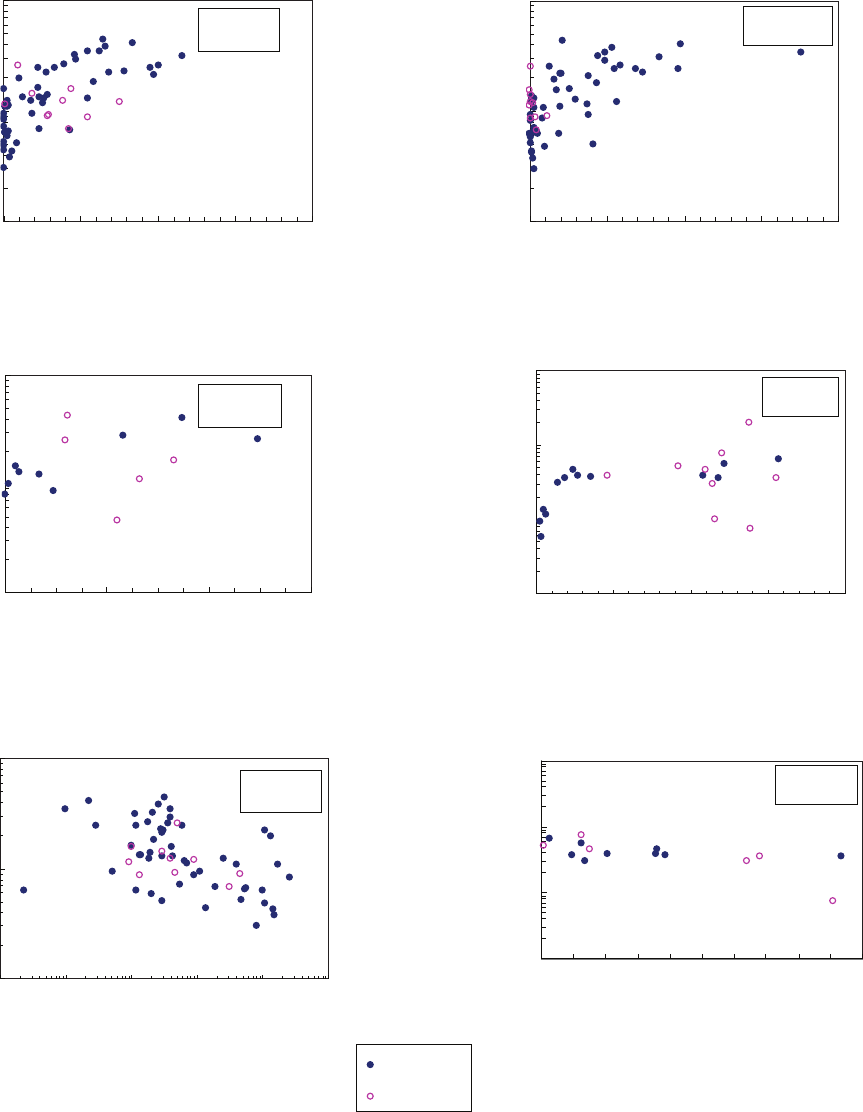
36 Mercury in Fish, Bed Sediment, and Water from Streams Across the United States, 1998–2005
11-7093-c_fig 21a-f
0.1
1
10
0 20 40 60 80
Largemouth bass
0.1
1
10
0 20 40 60 80
EVERGREEN FOREST, PERCENT OF BASIN AREA,
DISTANCE-WEIGHTED
EVERGREEN FOREST, PERCENT OF BASIN AREA,
DISTANCE-WEIGHTED
TOTAL MERCURY IN FISH,
MICROGRAMS PER GRAM PER METER
TOTAL MERCURY IN FISH,
MICROGRAMS PER GRAM PER METER
TOTAL MERCURY IN FISH,
MICROGRAMS PER GRAM PER METER
TOTAL MERCURY IN FISH,
MICROGRAMS PER GRAM PER METER
TOTAL MERCURY IN FISH,
MICROGRAMS PER GRAM PER METER
TOTAL MERCURY IN FISH,
MICROGRAMS PER GRAM PER METER
Unmined
Mined
r
s
= 0.77
p < 0.001
WOODY WETLAND, PERCENT OF BASIN AREA,
DISTANCE-WEIGHTED
EVERGREEN FOREST, PERCENT OF BASIN AREA,
DISTANCE-WEIGHTED
p < 0.001
B
0.01
0.1
1
10
0 20 40 60 80
p < 0.001
Brown trout
D
0.1
1
10
0 20 40 60
p < 0.05
Spotted bass
C
0.1
1
10
0.1 1 10 100 1000 10000
POPULATION DENSITY,
PEOPLE PER SQUARE KILOMETER
POPULATION DENSITY,
PEOPLE PER SQUARE KILOMETER
p < 0.001
Largemouth bass
E
0.01
0.1
1
10
0 1 2 3 4 5 6 7 8 9 10
p < 0.01
Brown trout
F
A
Largemouth bass
r
s
= 0.72
r
s
= -0.50
r
s
= 0.72
r
s
= 0.86
r
s
= -0.75
Figure 21. Correlations between length-normalized mercury concentrations in fish and selected environmental
characteristics, 1998–2005. [Data for all sites shown, unmined and mined; however, Spearman rank correlation
coefficients (r
s
) are for unmined sites only.]

Factors Related to Mercury Bioaccumulation in Fish 37
11-7093-c_fig 21g-l
0.1
1
10
0.01 0.1 1
p = 0.10
Spotted bass
H
0.1
1
10
0 1 10 100
METHYLMERCURY IN BED SEDIMENT,
NANOGRAMS PER GRAM
p < 0.01
J
Pumpkinseed
0.1
1
10
0.01 0.1 1
p < 0.05
Largemouth bass
G
0.01
0.1
1
10
0.01 0.1 1
p < 0.05
Rainbow-Cutthroat trout
I
0.1
1
10
0 1 10 100
p < 0.001
L
Pumpkinseed
0.01
0.1
1
10
0.01 0.1 1 10 100
METHYLMERCURY AS A PERCENTAGE
OF TOTAL MERCURY IN BED SEDIMENT
METHYLMERCURY AS A PERCENTAGE
OF TOTAL MERCURY IN BED SEDIMENT
p < 0.05
Brown trout
K
METHYLMERCURY IN BED SEDIMENT, NANOGRAMS
PER GRAM, DIVIDED BY PERCENT LOSS ON IGNITION
METHYLMERCURY IN BED SEDIMENT, NANOGRAMS
PER GRAM, DIVIDED BY PERCENT LOSS ON IGNITION
METHYLMERCURY IN BED SEDIMENT, NANOGRAMS
PER GRAM, DIVIDED BY PERCENT LOSS ON IGNITION
TOTAL MERCURY IN FISH,
MICROGRAMS PER GRAM PER METER
TOTAL MERCURY IN FISH,
MICROGRAMS PER GRAM PER METER
TOTAL MERCURY IN FISH,
MICROGRAMS PER GRAM PER METER
TOTAL MERCURY IN FISH,
MICROGRAMS PER GRAM PER METER
TOTAL MERCURY IN FISH,
MICROGRAMS PER GRAM PER METER
TOTAL MERCURY IN FISH,
MICROGRAMS PER GRAM PER METER
Unmined
Mined
r
s
= 0.35
r
s
= 0.60
r
s
= 0.67
r
s
= 0.74
r
s
= 0.56
r
s
= 0.85
Figure 21.—Continued.

38 Mercury in Fish, Bed Sediment, and Water from Streams Across the United States, 1998–2005
11-7093-c_fig 21m-r
0.1
1
10
0.01 0.1 1
Pumpkinseed
0.01
0.1
1
10
0.001 0.01 0.1 1 10
WHMI.5
DELR.26
N
Smallmouth bass
0.1
1
10
0.01 0.1 1 10
Largemouth bass
M
0.1
1
10
0.1 1 10 100
Largemouth bass
O
0.1
1
10
0.1 1 10
R
Pumpkinseed
0.01
0.1
1
10
0.1 1 10
Rainbow-Cutthroat trout
Q
P
Unmined
Mined
TOTAL MERCURY IN FISH,
MICROGRAMS PER GRAM PER METER
TOTAL MERCURY IN FISH,
MICROGRAMS PER GRAM PER METER
TOTAL MERCURY IN FISH,
MICROGRAMS PER GRAM PER METER
TOTAL MERCURY IN FISH,
MICROGRAMS PER GRAM PER METER
TOTAL MERCURY IN FISH,
MICROGRAMS PER GRAM PER METER
TOTAL MERCURY IN FISH,
MICROGRAMS PER GRAM PER METER
METHYLMERCURY IN UNFILTERED WATER,
NANOGRAMS PER LITER
METHYLMERCURY IN UNFILTERED WATER,
NANOGRAMS PER LITER
METHYLMERCURY IN UNFILTERED WATER,
NANOGRAMS PER LITER
TOTAL MERCURY IN UNFILTERED WATER,
NANOGRAMS PER LITER
TOTAL MERCURY IN UNFILTERED WATER,
NANOGRAMS PER LITER
TOTAL MERCURY IN UNFILTERED WATER,
NANOGRAMS PER LITER
r
s
= 0.50
r
s
= 0.79
r
s
= 0.54
r
s
= -0.52
r
s
= 0.37
r
s
= 0.19
p < 0.01
p > 0.10
p < 0.001
p < 0.01
p < 0.05
p < 0.05
Figure 21.—Continued.

Factors Related to Mercury Bioaccumulation in Fish 39
11-7093-c_fig 21s_x
0.01
0.1
1
10
1 10 100
DISSOLVED SULFATE IN UNFILTERED WATER,
MILLIGRAMS PER LITER
Brown trout
T
0.1
1
10
0.1 1 10 100 1000
DISSOLVED SULFATE IN UNFILTERED WATER,
MILLIGRAMS PER LITER
Largemouth bass
S
0.01
0.1
1
10
1 10 100
DISSOLVED ORGANIC CARBON IN UNFILTERED WATER,
MILLIGRAMS PER LITER
Brown trout
V
0.1
1
10
1 10
SPECIFIC ULTRAVIOLET ABSORBANCE OF UNFILTERED WATER
AT 254 NANOMETERS, LITER PER MILLIGRAMS CARBON PER METER
Largemouth bass
W
0.1
1
10
4 5 6 7 8 9 10
PH, UNFILTERED WATER
Largemouth bass
U
0.1
1
10
1 10 100
TOTAL MERCURY IN ATMOSPHERIC DEPOSITION,
SEIGNEUR-MODELED, WET AND DRY, MICROGRAMS PER SQUARE METER
Rock bass
X
TOTAL MERCURY IN FISH,
MICROGRAMS PER GRAM PER METER
TOTAL MERCURY IN FISH,
MICROGRAMS PER GRAM PER METER
TOTAL MERCURY IN FISH,
MICROGRAMS PER GRAM PER METER
TOTAL MERCURY IN FISH,
MICROGRAMS PER GRAM PER METER
TOTAL MERCURY IN FISH,
MICROGRAMS PER GRAM PER METER
TOTAL MERCURY IN FISH,
MICROGRAMS PER GRAM PER METER
Unmined
Mined
p < 0.001
p < 0.01
r
s
= -0.54
r
s
= -0.43
r
s
= 0.71
r
s
= 0.76
r
s
= -0.60
r
s
= -0.60
p < 0.001
p < 0.05
p < 0.001
p < 0.001
Figure 21.—Continued.

40 Mercury in Fish, Bed Sediment, and Water from Streams Across the United States, 1998–2005
For the 1998 National Mercury Pilot, Brumbaugh and
others (2001) showed a highly signicant correlation between
length-normalized Hg in largemouth bass and MeHg in
unltered water (r
s
= 0.71, p < 0.001). In our study, sh-Hg
concentrations also correlated positively with unltered MeHg
for largemouth bass (r
s
= 0.50; g. 21M) and pumpkinseed
(r
s
= 0.79; g. 21O), but the relation was not signicant for
smallmouth bass (g. 21N) or other sh species evaluated
(table 5). Fish Hg appeared to be similarly correlated with
ltered MeHg concentrations; however, some correlations
with this parameter must be viewed with caution because
ltered Hg data were available at far fewer sites than unltered
Hg data, and concentrations at many of these sites were below
detection limits. Fish Hg also correlated with THg in unltered
water, but generally more weakly than to MeHg; this relation
was positive for largemouth bass and rainbow-cutthroat
trout, and was negative for pumpkinseed (gs. 21P–21R).
Total Hg in ltered samples appeared to be a better predictor
of spotted bass Hg concentrations than MeHg in unltered
water, although it is MeHg in water that is accumulated in the
aquatic food web eventually to sh. Noise in the correlations
with MeHg in unltered water might be reduced with
increased water sampling, such as was done by Chasar and
others (2009). Multiple samples over a range of hydrologic
conditions, and possibly lower detection limits, would be
needed to improve correlations.
In general, length-normalized Hg concentrations in
sh correlated weakly to selected ancillary water chemistry
characteristics. Fish Hg in largemouth bass and brown
trout were negatively correlated with concentrations of
dissolved sulfate in water (gs. 21S, 21T). Sulfate may
exert concentration-dependent positive or negative effects
on Hg methylation and, therefore, bioaccumulation by sh
(Compeau and Bartha, 1983, 1987; Gilmour and others,
1992, 1998; Benoit and others, 2003). A negative correlation
with pH was found for Hg in largemouth bass only (r
s
=
-0.43; g. 21U). Lower pH waters (more acidic) tend to be
associated with a greater partitioning of Hg to the dissolved
phase, enhancing Hg methylation, and resulting in higher rates
of Hg bioaccumulation (Watras and Bloom, 1992). Although
DOC and sh Hg directly correlated only in rock bass (table 5)
and brown trout (g. 21V), water BAF values for largemouth
bass and brown trout decreased with increasing concentrations
of DOC in unltered water (gs. 22G, H). In contrast, Hg in
largemouth bass positively correlated with SUVA of DOC
(g. 21W). This supports the importance of the indirect
and positive effect of DOC and DOC complexity in sh Hg
bioaccumulation, as also found by Chasar and others (2009)
for DOC and SUVA for top-predator sh.
With the exception of rock bass, no relation was
found between atmospheric THg deposition and sh-Hg
concentrations when examined at sites across the United
States (g. 21X); however, variation in local environmental
characteristics in stream basins may confound evidence of
the potential effects of atmospheric deposition. The three
bass species that are widespread in the eastern half of the
United States (largemouth, smallmouth, and rock bass) were
examined further for relations to atmospheric THg deposition
by conning analyses to sites from mixed and undeveloped
LULC; sites from mined, urban, and agricultural LULC were
excluded to minimize confounding effects of nonatmospheric
Hg sources and land-use disturbances. Length-normalized
Hg in sh was compared to three estimates of Hg deposition:
total combined [sum of precipitation-weighted wet THg
deposition measured at MDN sites and modeled dry THg
deposition (Seigneur and others, 2004)]; total modeled [sum
of modeled wet and dry THg deposition from Seigneur and
others (2004)]; and wet only [precipitation-weighted wet THg
deposition measured at MDN sites]. In addition to the positive
correlation mentioned earlier for total modeled Hg deposition
with rock bass (g. 21X), total combined deposition positively
correlated with rock bass Hg (not shown). The positive
relation for rock bass Hg with Hg deposition also remained
signicant in the multiple regression model that included
evergreen forest and woody wetland abundance. Relations
between largemouth bass Hg levels and either total combined
or wet only Hg deposition were deemed not reliable because
four inuential samples were in Kansas and Nebraska, where
the western U.S. average was used as an estimate of Hg
deposition. Given the lack of wet deposition measurements
in that part of the country we do not have condence in the
accuracy of this estimate for Kansas and Nebraska. When the
four low-Hg deposition samples were excluded, there was
no signicant relation. Relations for smallmouth bass with
atmospheric Hg were not signicant.
Hammerschmidt and Fitzgerald (2006) examined a large,
historical data set for 25 States and found positive relations
between statewide average Hg in largemouth bass and wet
Hg deposition. Our site-based (rather than statewide) analysis
provides limited support for positive relation between sh-Hg
concentration and Hg deposition. One explanation for the
limited connection between Hg in sh and deposition in our
study is that variation in Hg methylation among ecosystems is
greater than the variation in Hg deposition, particularly in the
eastern United States, where most of our bass were sampled.

Factors Related to Mercury Bioaccumulation in Fish 41
11-7093-c_fig 22a-f
0.01 0.1 1 10 100
LOSS ON IGNITION OF BED SEDIMENT, PERCENT
LOSS ON IGNITION OF BED SEDIMENT, PERCENT
LOSS ON IGNITION OF BED SEDIMENT, PERCENT
LOSS ON IGNITION OF BED SEDIMENT, PERCENT
LOSS ON IGNITION OF BED SEDIMENT, PERCENT
LOG SEDIMENT-FISH
BIOTA ACCUMULATION FACTOR
LOG SEDIMENT-FISH
BIOTA ACCUMULATION FACTOR
LOG SEDIMENT-FISH
BIOTA ACCUMULATION FACTOR
LOG SEDIMENT-FISH
BIOTA ACCUMULATION FACTOR
LOG SEDIMENT-FISH
BIOTA ACCUMULATION FACTOR
LOG SEDIMENT-FISH
BIOTA ACCUMULATION FACTOR
Largemouth bass
A
0.1 1 10
Spotted bass
C
1
2
3
4
5
6
1
2
3
4
5
6
1
2
3
4
5
6
1
2
3
4
5
6
1
2
3
4
5
6
1
2
3
4
5
6
0.1 1 10 100
Rock bass
B
0.1 1 10 100
Brown trout
D
0.1 1 10 100
Rainbow-Cutthroat trout
E
0.001 0.01 0.1 1 10 100 1000
ACID VOLATILE SULFIDE IN BED SEDIMENT,
MICROGRAMS PER GRAM
DRY WEIGHT
Largemouth bass
F
Unmined
Mined
p < 0.0001
p < 0.01
r
s
= -0.63
r
s
= -0.30
p> 0.10
r
s
= -0.85
r
s
= -0.78
r
s
= -0.55
p > 0.10
r
s
= -0.63
p < 0.01
p < 0.001
Figure 22. Biota Accumulation Factors (BAF) for fish in relation to selected environmental characteristics,
1998–2005. [Data for all sites are shown, unmined and mined; however, Spearman rank correlation coefficients
(r
s
) are for unmined only. BAF values are in Log
10
.]

42 Mercury in Fish, Bed Sediment, and Water from Streams Across the United States, 1998–2005
Bed-Sediment Relations with
Environmental Characteristics
Higher concentrations of MeHg in bed sediment at
sites in unmined basins (n = 183) were signicantly related
to higher LOI, THg, and AVS of the sediment, as shown in
equation 3 (adjusted r
2
= 0.73):
BS
BS
BS
ln[MeHg ] = - 2.857 + 0.925 ln[LOI]
+ 0.247 ln[THg ] 0.048 ln[AVS] ,
where
MeHg is the bed sediment MeHg concentration,
in nanograms per gram,
LOI is the loss-on-ignition of the bed sediment
in percent,
T
+
BS
Hg is the bed sediment THg concentration, in
nanograms per gram, and
AVS is the acid-volatile sulfide concentration,
in micrograms per gram.
(3)
LOI was a strong predictor of MeHg in bed sediment
(r
s
= 0.81, g. 23A) and THg in bed sediment (r
s
=0.78;
table 6). Although bed sediment MeHg was near or below
detection at many sites, MeHg and THg were more highly
related in bed sediment (r
s
= 0.72) (g. 23B, table 6) than in
unltered water (r
s
= 0.40). Krabbenhoft and others (1999)
also found a high positive correlation between bed sediment
MeHg and LOI, as well as with sediment organic carbon.
Recent work by Marvin-DiPasquale and others (2009) found
that MeHg in bed sediment from streams with predominantly
atmospheric Hg inputs was a function of sediment organic
content and the activity of Hg-methylating microbes. AVS
correlated positively with bed sediment MeHg and THg in our
study (g. 23C) but contributed least to the predictive power
of equation 3. Key LULC categories, such as forest cover,
wetland, urban, and agriculture, were at most only weakly
correlated with Hg concentrations in bed sediment (table 6).
As atmospheric Hg concentrations increased,
concentrations of THg in bed sediment increased, and the
highest correlation (r
s
= 0.53) was found for Seigneur-modeled
dry atmospheric deposition with bed sediment THg (g. 23D;
table 6); the correlation between THg and Seigneur-modeled
total (wet + dry) atmospheric deposition was lower, but still
signicant (r
s
= 0.39).
11-7093-c_fig 22g-h
4
5
6
7
8
9
0.1 1 10 100
DISSOLVED ORGANIC CARBON IN UNFILTERED WATER,
MILLIGRAMS PER LITER
LOG WATER-FISH BIOTA
ACCUMULATION FACTOR
Brown trout
H
G
Largemouth bass
4
5
6
7
8
9
0.1 1 10 100
DISSOLVED ORGANIC CARBON IN UNFILTERED WATER,
MILLIGRAMS PER LITER
LOG WATER-FISH BIOTA
ACCUMULATION FACTOR
r
s
= -0.58
p < 0.001
r
s
= -0.63
p < 0.01
Mined
Non-mined
Figure 22.—Continued

Bed-Sediment Relations with Environmental Characteristics 43
Figure 23. Correlations between mercury in bed sediment and selected environmental characteristics
in unmined basins, 1998–2005. (r
s
, Spearman rank correlation coefficient; modeled mercury is based on
Seigneur and others, 2004.)
0.001
0.010
0.100
1.000
10.000
100.000
0.001 0.1 10 1000 100000
ACID-VOLATILE SULFIDE IN BED SEDIMENT,
IN MICROGRAMS PER GRAM DRY WEIGHT
C
r
s
= 0.46
p < 0.001
0.001
0.010
0.100
1.000
10.000
100.000
0.1 1 10 100
LOSS-ON-IGNITION OF BED SEDIMENT,
PERCENT
METHYLMERCURY IN BED SEDIMENT,
NANOGRAMS PER GRAM DRY WEIGHT
METHYLMERCURY IN BED SEDIMENT,
NANOGRAMS PER GRAM DRY WEIGHT
TOTAL MERCURY IN BED SEDIMENT,
NANOGRAMS PER GRAM DRY WEIGHT
METHYLMERCURY IN BED SEDIMENT,
NANOGRAMS PER GRAM DRY WEIGHT
r
s
= 0.81
p < 0.0001
A
0.001
0.010
0.100
1.000
10.000
100.000
0.1 1 10 100 1000 10000
TOTAL MERCURY IN BED SEDIMENT,
NANOGRAMS PER GRAM DRY WEIGHT
r
s
= 0.72
p < 0.0001
B
0.1
1
10
100
1000
10000
1 10 100
TOTAL MERCURY IN ATMOSPHERIC DEPOSITION,SEIGNEUR-
MODELED, DRY ONLY, MICROGRAMS PER SQUARE METER
D
r
s
= 0.53
p< 0.001
11-7093-c_fig 23a-d

44 Mercury in Fish, Bed Sediment, and Water from Streams Across the United States, 1998–2005
Table 6. Spearman rank correlation coefficients (r
s
) for relations between selected environmental characteristics from U.S. streams, 1998–2005.
[Denitions of variable abbreviations are listed in Appendix 1. Values are for sites in unmined basins only. Color coding of r
s
based on p values, p < 0.001 (pink), p < 0.01 (orange), and p < 0.05 (yellow)]
Parameter pH DOC UV SUVA Sulfate
SS_
conc
UMeHg UTHg
UMeHg/
UTHg
FMeHg FTHg PMeHg PTHg
SMeHg/
LOI
SMeHg
STHg /
LOI
STHg
SMeHg/
STHg
LOI AVS
Stream water
pH 1.00
DOC -0.23 1.00
UV -0.24 0.92 1.00
SUVA -0.55 0.31 0.60 1.00
Sulfate 0.40 0.12 -0.16 -0.45 1.00
SS_conc 0.09 0.36 -0.22 0.05 0.27 1.00
UMeHg -0.39 0.59 0.67 0.47 -0.09 0.55 1.00
UTHg -0.23 0.43 0.31 0.28 0.14 0.62 0.54 1.00
UMeHg/UTHg -0.29 0.37 0.48 0.30 -0.26 0.13 0.72 -0.12 1.00
FMeHg -0.31 0.56 0.51 0.42 0.07 0.26 0.83 0.50 0.58 1.00
FTHg -0.31 0.49 0.31 0.31 0.03 0.27 0.61 0.79 0.04 0.67 1.00
PMeHg -0.07 0.31 0.03 -0.06 0.40 0.69 0.77 0.72 0.22 0.46 0.45 1.00
PTHg -0.08 0.15 0.04 -0.16 0.42 0.61 0.45 0.79 -0.29 0.19 0.36 0.72 1.00
Bed sediment
SMeHg/LOI -0.20 0.03 -0.15 0.16 0.01 0.07 0.28 0.23 0.14 0.27 0.21 0.36 0.21 1.00
SMeHg -0.28 0.08 -0.06 0.28 -0.13 0.15 0.28 0.16 0.19 0.09 0.11 0.31 0.17 0.77 1.00
STHg/LOI -0.05 0.10 -0.21 -0.19 0.33 -0.01 -0.08 0.29 -0.33 0.13 0.26 0.14 0.34 0.26 0.08 1.00
STHg -0.25 0.16 -0.03 0.14 0.02 0.05 0.10 0.22 -0.08 0.02 0.17 0.17 0.27 0.39 0.72 0.51 1.00
SMeHg/STHg -0.08 -0.07 -0.04 0.19 -0.23 0.07 0.31 -0.03 0.39 0.09 -0.04 0.16 -0.12 0.63 0.59 -0.50 -0.06 1.00
LOI -0.28 0.13 0.12 0.31 -0.22 0.05 0.21 0.07 0.18 -0.02 0.00 0.12 0.03 0.29 0.81 -0.08 0.78 0.30 1.00
AVS -0.27 0.14 0.42 0.32 0.03 0.07 0.08 0.14 -0.03 0.09 0.16 0.14 0.04 0.31 0.46 0.17 0.40 0.13 0.42 1.00
Atmospheric deposition
SULF.DEP -0.08 -0.03 -0.21 -0.03 0.32 -0.16 -0.08 -0.03 -0.12 0.35 0.19 0.18 0.20 0.24 0.17 0.44 0.28 -0.11 0.05 0.17
ADRY.SEI -0.20 0.10 -0.21 -0.09 0.29 -0.20 0.01 -0.01 -0.04 0.25 0.09 0.10 0.15 0.36 0.42 0.44 0.53 -0.03 0.35 0.26
ATOT.SEI -0.16 -0.06 -0.28 -0.15 0.22 -0.39 -0.12 -0.09 -0.12 0.06 -0.03 -0.11 -0.03 0.25 0.25 0.45 0.39 -0.12 0.19 0.12
AWET.MDN -0.04 0.07 0.13 0.23 0.17 -0.08 -0.10 0.00 -0.12 0.36 0.11 0.03 -0.00 -0.16 -0.37 0.21 -0.27 -0.24 -0.44 -0.13
AWET.PRE -0.07 0.13 0.18 0.27 0.20 0.03 -0.05 0.01 -0.06 0.37 0.12 0.12 0.03 -0.11 -0.26 0.18 -0.18 -0.18 -0.31 -0.09
PREC.PR -0.45 -0.04 0.12 0.33 -0.35 -0.49 -0.03 -0.05 0.03 0.13 0.09 -0.31 -0.22 0.05 0.02 0.22 0.15 -0.10 0.06 0.06
WET_DEP_AVE 0.24 -0.51 -0.50 -0.19 -0.18 -0.07 -0.27 -0.16 -0.20 -0.44 -0.26 -0.13 -0.09 -0.08 -0.02 -0.23
-0.10 0.10 0.02 -0.09
Other
POPDEN00 -0.11 0.28 0.23 0.04 0.42 -0.04 0.01 0.14 -0.14 0.13 0.08 0.10 0.34 0.11 0.15 0.47 0.40 -0.25 0.17 0.18
ELEV.AVG 0.54 -0.41 -0.52 -0.53 0.01 0.01 -0.31 -0.17 -0.24 -0.37 -0.15 -0.08 -0.08 -0.02 -0.05 -0.26 -0.21 0.15 -0.12 -0.14
HYDRIC SOILS -0.22 0.48 0.56 0.35 0.06 0.11 0.31 0.09 0.28 0.36 0.19 0.09 -0.06 0.04 0.01 0.13 0.05 -0.04 -0.01 0.04
PET -0.14 0.18 0.32 0.25 0.28 0.17 0.12 0.18 0.00 0.31 0.11 0.21 0.22 -0.26 -0.42 0.10 -0.30 -0.27 -0.40 -0.11
AET -0.25 0.18 0.28 0.34 0.18 0.04 0.10 0.12 0.04 0.37 0.16 0.12 0.10 -0.18 -0.32 0.17 -0.17 -0.25 -0.30 -0.10

Bed-Sediment Relations with Environmental Characteristics 45
Parameter pH DOC UV SUVA Sulfate
SS_
conc
UMeHg UTHg
UMeHg/
UTHg
FMeHg FTHg PMeHg PTHg
SMeHg/
LOI
SMeHg
STHg /
LOI
STHg
SMeHg/
STHg
LOI AVS
Land use / land cover
SUM_FOREST -0.26 -0.19 -0.30 0.11 -0.56 -0.41 -0.04 -0.15 0.10 0.03 0.15 -0.30 -0.41 0.18 0.30 -0.15 0.18 0.27 0.31 0.02
EVR_FOREST -0.32 -0.16 -0.10 0.23 -0.68 -0.30 0.03 -0.08 0.14 -0.04 0.09 -0.38 -0.47 0.04 0.05 -0.25 -0.07 0.23 0.08 -0.10
EVR_FOREST_DW -0.32 -0.16 -0.14 0.21 -0.68 -0.30 0.05 -0.08 0.17 -0.01 0.10 -0.35 -0.45 0.05 0.07 -0.29 -0.08 0.26 0.09 -0.12
SUM_WETLAND -0.45 0.49 0.66 0.55 -0.22 0.19 0.47 0.18 0.41 0.38 0.24 0.15 -0.05 0.09 0.17 -0.02 0.13 0.09 0.21 0.20
WOODWETLAND -0.50 0.47 0.58 0.58 -0.25 0.09 0.42 0.15 0.37 0.43 0.29 0.06 -0.12 0.10 0.17 0.05 0.17 0.07 0.21 0.20
WOODWETLAND_DW -0.51
0.45 0.55 0.57 -0.26 0.15 0.44 0.19 0.37 0.44 0.29 0.10 -0.09 0.08 0.14 0.02 0.14 0.07 0.20 0.19
HERBWETLAND -0.22 0.51 0.67 0.35 -0.06 0.19 0.39 0.14 0.37 0.21 0.10 0.17 0.02 0.12 0.25 -0.02 0.25 0.07 0.32 0.21
HERBWETLAND_DW -0.23 0.52 0.70 0.38 -0.06 0.21 0.39 0.15 0.36 0.22 0.11 0.18 0.01 0.11 0.23 0.00 0.24 0.05 0.29 0.24
SUM_UNDEVELOPED -0.16 -0.17 -0.13 0.13 -0.62 -0.19 0.07 -0.10 0.19 -0.05 0.09 -0.13 -0.38 0.12 0.17 -0.34 -0.03 0.32 0.19 -0.00
SUM_URBAN -0.14 0.28 0.21 0.05 0.39 0.00 0.07 0.16 -0.11 0.18 0.11 0.16 0.36 0.15 0.16 0.45 0.38 -0.21 0.15 0.18
RES_L_URBAN -0.17 0.29 0.20 0.05 0.40 -0.02 0.08 0.18 -0.09 0.18 0.08 0.16 0.35 0.17 0.18 0.49 0.41 -0.22 0.17 0.19
RES_L_URBAN_DW -0.15 0.29 0.17 -0.02 0.40 -0.01 0.08 0.18 -0.09
0.19 0.10 0.17 0.36 0.19 0.20 0.52 0.42 -0.21 0.16 0.18
RES_H_URBAN -0.07 0.26 0.23 0.06 0.46 0.02 -0.05 0.18 -0.23 0.14 0.06 0.05 0.24 0.03 -0.02 0.45 0.21 -0.32 -0.02 0.10
RES_H_URBAN_DW -0.05 0.26 0.22 0.00 0.46 0.02 -0.05 0.18 -0.23 0.15 0.06 0.06 0.24 0.04 -0.00 0.46 0.22 -0.31 -0.02 0.09
COM_INDUSTR -0.12 0.33 0.27 0.09 0.40 0.12 0.11 0.20 -0.08 0.17 0.16 0.20 0.40 0.09 0.13 0.41 0.35 -0.22 0.15 0.16
COM_INDUSTR_DW -0.12 0.30 0.20 -0.01 0.39 0.11 0.10 0.18 -0.10 0.18 0.17 0.21 0.42 0.13 0.14 0.43 0.35 -0.21 0.13 0.12
SUM_AGRICULTURE 0.19 0.05 -0.08 -0.11 0.43 0.30 -0.02 0.07 -0.09 0.10 -0.02 0.25 0.32 -0.14 -0.21 0.06 -0.17 -0.09 -0.25 -0.14
ROW_CROP 0.01 0.15 -0.00 -0.00 0.29 0.32 0.14 0.14 0.06 0.18 0.02 0.29 0.29 0.01 -0.05 0.04 -0.09
0.05 -0.13 -0.13
ROW_CROP_DW 0.00 0.15 0.00 0.01 0.27 0.32 0.15 0.12 0.09 0.17 -0.00 0.27 0.27 0.04 -0.03 0.02 -0.08 0.09 -0.12 -0.12
PAST_HAY 0.20 -0.01 -0.17 -0.15 0.41 0.23 -0.11 0.07 -0.20 0.19 0.09 0.24 0.37 -0.19 -0.23 0.11 -0.13 -0.17 -0.23 -0.17
PAST_HAY_DW 0.23 -0.04 -0.16 -0.13 0.39 0.23 -0.12 0.05 -0.20 0.16 0.07 0.20 0.32 -0.18 -0.24 0.07 -0.17 -0.14 -0.26 -0.19
GRASSLAND 0.39 -0.05 0.12 -0.17 0.04 0.33 -0.07 0.02 -0.05 -0.27 -0.12 0.10 0.04 -0.30 -0.30 -0.34 -0.39 0.00 -0.23 -0.14
Table 6. Spearman rank correlation coefficients (r
s
) for relations between selected environmental characteristics from U.S. streams, 1998–2005.—Continued
[Denitions of variable abbreviations are listed in Appendix 1. Values are for sites in unmined basins only. Color coding of r
s
based on p values, p < 0.001 (pink), p < 0.01 (orange), and p < 0.05 (yellow)]

46 Mercury in Fish, Bed Sediment, and Water from Streams Across the United States, 1998–2005
Stream-Water Relations with
Environmental Characteristics
Stepwise multiple-linear regression indicated that higher
concentrations of MeHg in unltered water from sites in
unmined basins (n = 223) were primarily related to higher
DOC and THg of unltered stream water and, to a lesser
extent, higher percentages of MeHg in bed sediment, higher
percentages of total wetland (woody and herbaceous) in the
basin, and lower pH values of the water (adjusted r
2
= 0.61):
water
water
BS
w
water
ln[MeHg ] = - 1.664 + 0.573 ln[DOC]
+ 0.384 ln[THg ] 0.270 [pH]
+ 0.268 ln[MeHg/THg ]
+ 0.015 arcsin[L ],
where
MeHg is the MeHg concentration in unfiltered
water, in nanograms per lit
−
BS
water
er,
DOC is the dissolved organic carbon
concentration in unfiltered water, in
milligrams per liter,
MeHg / THg is the percentage of MeHg in bed
sediment,
THg is the THg concentration in unfiltered
water, i
w
n nanograms per liter, pH is
the pH value in unfiltered water, and
L is the percentage of total wetland in the
basin.
(4)
MeHg concentrations in unltered water correlated
positively with concentrations of DOC (r
s
= 0.59, p < 0.001)
and UV absorbance (r
s
= 0.67, p < 0.001) (g. 24A, 24B;
table 6). UV absorbance has been suggested as an inexpensive
surrogate measure for Hg concentration in water because it
correlates highly with DOC and even more highly with the
types of DOC thought to complex most strongly with Hg
(George R. Aiken, U.S. Geological Survey, oral commun.,
2003). The correlation of unltered MeHg to SUVA (r
s
=
0.466, p < 0.01) was not as strong. Similar but weaker
correlations were found between ltered MeHg concentrations
and DOC, UV absorbance, and SUVA. DOC, in turn,
correlated positively with hydric soils, total wetness index,
total wetlands, and precipitation-weighted atmospheric Hg
deposition, and it correlated negatively with average basin
elevation and average depth to the seasonally high water table.
Spearman correlations between MeHg and THg in water
ranged from r
s
= 0.54 in unltered water (g. 24C) to r
s
= 0.72
in particulate water samples (table 6). In addition, MeHg and
THg in unltered and particulate samples increased in relation
to total suspended-sediment concentration. A weak negative
relation was found between MeHg and pH in unltered water
(g. 24D). The percentage of MeHg (percent MeHg/THg) in
unltered water was positively correlated with percent MeHg
in bed sediment (g. 24E).
MeHg concentrations in unltered water were higher
at sites in basins with higher percentages of total wetland
(g. 24F) and with both woody wetland and herbaceous
wetland (table 6). Increasing percentages of hydric soils were
only weakly predictive of unltered MeHg. Other LULC and
basin-level GIS measured characteristics were limited in their
value for explaining Hg in water.
No correlation was found for modeled or actual Hg from
atmospheric deposition with unltered MeHg; however, this
is not surprising, given that water samples were collected only
once at each site. The analysis was also hampered for ltered
MeHg by many values below reporting limits and by sparse
NADP-MDN wet-deposition data for Western States.
Discussion of Findings and Comparison
with Other Studies
Our results for total Hg in sh provide evidence that
Hg concentrations in freshwater sh across the United
States are often greater than levels specied in various
criteria for protection of sh-eating wildlife and humans.
However, the purpose of our study was to compare sites
and explore factors related to sh Hg; it was not intended to
be a thorough assessment of sh Hg with respect to sh-
consumption-advisory levels. The results presented here
paint a picture of Hg in streams across the United States for
a broad range of regional and national gradients in Hg source
strength and factors thought to inuence Hg methylation and
bioaccumulation. Sources included atmospheric deposition,
urbanization, and gold or Hg mining; however, sampling
focused primarily on sites where atmospheric deposition was
the Hg source. Hg in sh, bed sediment, and stream water
were assessed spatially and with regard to existing guidelines
or criteria and possible relations to stream and basin attributes,
including chemical and physical characteristics, as well as
LULC. To date, there have been no other studies of this scale
in the literature that include multimedia sampling of MeHg
and THg and, currently, there is no national Hg monitoring
network in the United States for sh, bed sediment, and water.
A conceptual model for MeHg bioaccumulation is that
as MeHg is formed within the ecosystem through methylation
of inorganic Hg, some portion of the MeHg is transferred to
stream water, and some portion of MeHg in water is taken
up by the base of the aquatic food web through both sorption
to detritus and uptake into living algal (periphyton) cells.
MeHg is subsequently biomagnied in aquatic food webs

Discussion of Findings and Comparison with Other Studies 47
11-7093-c_fig 24
0.001
0.01
0.1
1
10
0.1 1 10 100
DISSOLVED ORGANIC CARBON,
MILLIGRAMS PER LITER
METHYLMERCURY
IN UNFILTERED WATER,
NANOGRAMS PER LITER
r
s
= 0.59
p < 0.0001
A
0.001
0.01
0.1
1
10
0.1 1 10 100
TOTAL MERCURY IN UNFILTERED WATER,
NANOGRAMS PER LITER
r
s
= 0.54
p < 0.001
r
s
= 0.39
p < 0.05
C
0.001
0.01
0.1
1
10
2 4 6 8 10 12
PH, UNFILTERED WATER
METHYLMERCURY
IN UNFILTERED WATER,
NANOGRAMS PER LITER
r
s
= -0.39
p < 0.001
D
METHYLMERCURY
IN UNFILTERED WATER,
NANOGRAMS PER LITER
0.001
0.01
0.1
1
10
0 20 40 60 80
TOTAL WETLAND, PERCENT OF BASIN AREA
METHYLMERCURY
IN UNFILTERED WATER,
NANOGRAMS PER LITER
r
s
= 0.46
p < 0.001
F
E
0.001
0.01
0.1
1
10
0.001 0.01 0.1 1 10
ULTRAVIOLET ABSORBANCE OF WATER AT 254
NANOMETERS, PER CENTIMETER
METHYLMERCURY
IN UNFILTERED WATER,
NANOGRAMS PER LITER
r
s
= 0.67
p < 0.001
B
0.1
1
10
100
0.01 0.1 1 10
METHYLMERCURY
IN UNFILTERED
WATER, AS PERCENT OF TOTAL MERCURY
METHYLMERCURY
IN STREAMBED SEDIMENT,
AS PERCENT OF TOTAL MERCURY
100
Figure 24. Correlations between mercury in unfiltered water and selected environmental characteristics in
unmined basins, 1998–2005. (r
s
, Spearman rank correlation coefficients.)
48 Mercury in Fish, Bed Sediment, and Water from Streams Across the United States, 1998–2005
to reach highest concentrations at the apex of the food web.
One plausible inference from this conceptual model is that
MeHg concentrations in organisms at the top of the aquatic
food web are linearly related to concentrations at the base of
the food web, which are in turn linearly related to aqueous
MeHg concentrations. We examined relations between sh
Hg, which is largely MeHg, to MeHg in water. Whereas sh
accumulate MeHg over time, MeHg in water is highly variable
over time, season, and hydrologic conditions. Our dataset
does not capture this variability, so correlations between sh
Hg and MeHg measured in this study are confounded by
the fact that single, instantaneous (single synoptic) aqueous
MeHg measurements are an uncertain estimator of longer-
term mean MeHg concentrations in a stream (Paller and
others, 2004; Brigham and others, 2009). Chasar and others
(2009), using temporally extensive water sampling and more
complete assessment of MeHg in aquatic food webs, support
the conceptual model that MeHg concentrations in predator
sh are related to mean aqueous MeHg concentrations and
that trophic transfer (biomagnication) is relatively consistent
among diverse stream ecosystems.
Concentrations of sh Hg from our study must be
compared to those from other studies with caution, owing
to inuences of sh species, age, length, weight, sex, and
sample cut or type (skin-off llets, as were most samples in
our study, compared to skin-on llets or whole-body sh). In
general, Hg increases with age and size in top-predator sh
and can be lower in whole-body sh compared to muscle
or llet. However, the ratio of llet to whole-body Hg may
be relatively consistent for some sh species (Boudou and
Ribeyre, 1983; Ribeyre and Boudou, 1984; Goldstein and
others, 1996). Differences in Hg relations with feeding
habitat, length, and weight have been noted in other large-
scale studies, including the historical NCBP (Schmitt and
others, 1999), the USGS BEST study (Schmitt, 2002; Schmitt
and others, 2004; Hinck and others, 2004a and 2004b, 2006,
2007), and USEPA EMAP (Peterson and others, 2007). For
example, Hinck and others (2004b) analyzed whole-body sh
from historical stream sites in major river basins of the United
States and found that piscivorous sh (bass and northern
pikeminnow) in the BEST Columbia River Basin study had
higher Hg concentrations than nonpiscivores and that Hg in
these sh increased with size.
Fish in streams receiving higher amounts of Hg due to
atmospheric load, gold or Hg mining, or urban contamination
have been found generally to have higher concentrations of
Hg. Hammerschmidt and Fitzgerald (2006) compared a large
historical dataset for Hg in largemouth bass (30-40 cm total
length) for 25 States with average annual wet atmospheric
deposition of Hg from the MDN and the literature for various
periods from the 1990s to early 2004. They excluded known
point sources and found a positive correlation between
statewide average concentrations of Hg in largemouth bass
and average annual wet deposition of Hg. Based on USEPA
EMAP results, Peterson and others (2007) suggested that
atmospheric deposition of Hg was an important source of sh
Hg in the western United States. However, at least one recent
paper found that effects of atmospheric deposition on sh Hg
were lessened by the structure and function of the particular
aquatic ecosystem (Rypel and others, 2008). They compared
largemouth bass in two river basins in the southeastern United
States; atmospheric Hg was not correlated with sh Hg. In
our study, we did not nd any relation to atmospheric THg
except for rock bass. In recent decades, industrial Hg use and
atmospheric Hg deposition have decreased in parts of the
United States (Engstrom and Swain, 1997). It is, therefore,
likely that sh-Hg concentrations are not at a steady state
but may be decreasing in the Nation’s waters. The response
time for sh Hg with regard to source input, such as from
atmospheric deposition, is unknown and is likely dependent on
many factors that were incompletely described or unmeasured
by this study.
Gold and Hg mining played an important role in
higher sh-Hg concentrations at selected sites in this
study, overwhelming correlations with other site or basin
characteristics. When sites in mined basins were excluded,
higher unltered MeHg in streams correlated with higher
unltered THg. Davis and others (2008) examined Hg in
largemouth bass and other sh in streams of the Sacramento-
San Joaquin Delta of California, an area affected by historical
gold and Hg mining. They found that the median sh Hg
for largemouth bass (0.53 µg/g ww) reected this inuence.
Detailed and accurate data on Hg sources, such as atmospheric
deposition, which is sparsely measured in the western
United States, as well as gold or Hg mining or other sources
of local Hg contamination, are critical to tease apart other
environmental characteristics contributing to Hg methylation
and sh Hg bioaccumulation.
In this study, the strongest correlations with
environmental characteristics were found for largemouth bass,
a top-predator/piscivorous sh, but signicant correlations
were also found for brown and rainbow-cutthroat trout, with
selected environmental characteristics that were often different
from those found for bass or other sunsh. In the USEPA
EMAP study, sh were also grouped by genera or family for
comparison to environmental factors (Peterson and others,
2007). Fish Hg for rainbow trout, cutthroat trout, and brown
trout genera, as well as for suckers, had the weakest relations,
if any, with measured environmental characteristics, whereas
top-predator/piscivorous genera, such as pikeminnow, had the
Discussion of Findings and Comparison with Other Studies 49
strongest. The interspecies differences we observed between
sh Hg correlations with environmental characteristics (for
example, largemouth and smallmouth bass) suggest caution
in generalizing beyond the species level. This concern has
been held historically for different groups of biota and other
environmental contaminants.
Results of the current study indicate that, if sites in gold
or Hg mined basins are excluded from statistical analysis, the
most important environmental characteristics for predicting
increasing concentrations of unltered MeHg in streams
are higher concentrations of DOC, unltered THg, and
bed-sediment MeHg, as well as higher basin percentages of
wetland and lower pH. Increased bed-sediment MeHg was
correlated with increasing LOI as a measure of sediment
organic content, bed-sediment THg, and AVS. The best
predictors of increasing sh Hg for largemouth bass were
increasing basin percentages of forest and wetland, MeHg
in unltered water and bed sediment, and decreasing pH and
dissolved sulfate. Although less important than water and
bed-sediment organic content (as measured by DOC and
LOI, respectively), sulfate was a useful characteristic for
understanding Hg in sh, bed sediment, and water. Dissolved
sulfate concentration negatively correlated with sh Hg for
largemouth bass and brown trout. Similarly, atmospheric
sulfate deposition positively correlated with sh Hg in rock
bass. The roles of pH and sulfate in Hg methylation have
been documented in the literature; sulfate is important in Hg
methylation by bacteria and, depending on concentration, can
have either a positive or negative effect on Hg methylation
(Compeau and Bartha, 1983, 1987; Gilmour and others, 1992,
1998; Benoit and others, 2003). The complex nature of sulfate
effects may help explain why it was not highly correlated
with sh Hg across the broad range of concentrations and
environmental conditions found in our study.
Increasing MeHg in water with increasing DOC, as found
in our study over a broad range of environmental conditions,
conrms similar results found in smaller scale studies with
regard to the role of DOC in Hg methylation (St. Louis and
others, 1994; Hurley and others, 1995). With the exception of
a negative correlation for rock bass, DOC was not correlated
with sh Hg, but unltered MeHg was found to be positively
correlated with sh Hg for all sh species where data were
sufcient for this examination. MeHg in unltered water was
less than 1 ng/L at most sites and, although MeHg in unltered
water was high for many sites in mined basins, both unltered
MeHg and sh Hg were high at many other sites that also
were high in DOC, such as coastal-plain streams along the
eastern and southern United States. These observations
underscore the importance of multiple factors that control Hg
bioaccumulation. A large source of Hg input to an ecosystem,
coupled with a modest capacity of the ecosystem to methylate
inorganic Hg, can produce high levels of MeHg in water and
sh. In contrast, a modest Hg source input to an ecosystem,
such as in ecosystems where atmospheric deposition is thought
to be the predominant source, coupled with a large capacity
of an ecosystem to methylate inorganic Hg, also can produce
high MeHg concentrations in water and sh.
High sh THg concentrations were found at sites that had
high percentages of forest and wetland, especially evergreen
forest and woody wetland more proximal to stream sites.
MeHg in unltered water positively correlated with wetland
abundance and, as for sh, MeHg relations to woody or
herbaceous wetland strengthened when these LULC types
were more proximal to stream sites. Wente (2000) showed
that proximity-based (distance-weighted) LULC explained
more variability in ecosystem integrity than more commonly
used standard percentages of LULC, a nding also seen
in this study. Other studies have found greater amounts of
wetland to be correlated with higher water MeHg (St. Louis
and others, 1994, 1996; Hurley and others, 1995; Krabbenhoft
and others, 1999; Grigal, 2002; Brigham and others, 2009).
Higher rates of Hg methylation in wetlands promote higher
MeHg in streams, especially during years of high water yield
(Krabbenhoft and others, 1995; Branreun and others, 1996).
Chumchal and others (2008) noted that Hg concentrations in
largemouth bass were higher from forested-wetland habitat
compared to open-water habitat. Our nding of higher
potential methylation rates, based on the MeHg to THg
ratio, at sites in basins with primarily undeveloped land in
comparison to urban land, agrees with ndings of Krabbenhoft
and others (1999) who noted that forested and mixed forest/
agricultural basins had higher rates than streams in mining
and urban basins. Horowitz and Stephens (2008) found that
THg in bed sediment was higher at sites in forested basins
(≥50 percent forested land use) than in basins in other LULC
categories. They analyzed data for a suite of trace elements
across 1,200 stream sites sampled as part of the NAWQA
Program during 1991 to 1999. Evergreen forest canopies have
greater effective surface areas than deciduous forest canopies
or open (non-forested) land for ltering Hg from atmospheric
deposition (Iverfeldt, 1991; Kolka and others, 1999). A study
by St. Louis and others (2001) showed that the tree canopies
of boreal forests receiving low atmospheric deposition are
signicant sources of both MeHg and THg via litter fall to the
forest oor, wetlands, and potentially to downstream water
bodies. This underscores the greater sensitivity and efciency
of these two LULC types with regard to Hg methylation.
50 Mercury in Fish, Bed Sediment, and Water from Streams Across the United States, 1998–2005
Summary and Conclusions
Hg in top-predator sh, bed sediment, and water was
examined from streams in diverse settings across the United
States during 1998–2005 by the USGS. Most studies of Hg
in aquatic environments have focused on lakes, reservoirs,
and wetlands because of the predominance of lakes with Hg
concerns and the importance of wetlands in Hg methylation.
Fewer studies have focused on Hg in streams or rivers. This
report describes the occurrence and distribution of THg in
stream sh in relation to regional and national gradients of Hg
source strength (including atmospheric deposition, gold and
Hg mining, urbanization) and other factors that are thought
to affect Hg concentrations, including LULC. In addition,
concentrations of THg and MeHg in bed sediment and stream
water were evaluated in relation to these gradients and to
identify ecosystem characteristics that favor the production
and bioaccumulation of MeHg.
Site selection targeted environmental settings thought
to be important with regard to the source, concentration,
or biogeochemical behavior of Hg in aquatic ecosystems.
Agricultural, urban, undeveloped (forested, grassland,
shrubland, and wetland land cover), and mined (for gold
and Hg) settings were of particular interest. Each site was
sampled one time during seasonal low ow. Predator sh
were targeted for collection, and composited skin-off llets
were analyzed for THg, as most of the Hg found in sh tissue
(95–99 percent) is MeHg. Bed sediment and stream water
were analyzed for THg, MeHg, and characteristics thought
to affect Hg methylation, such as LOI, AVS, pH, DOC, and
dissolved sulfate.
Key ndings of this report are as follows:
• Hg concentrations in sh at more than two-thirds of
the sites exceeded the value of 0.1 µg/g Hg ww that is
of concern for the protection of sh-eating mammals,
including mink and otters. Fish-Hg concentrations
equaling or exceeding the 0.3 µg/g ww USEPA
criterion for the protection of human health were found
at 27 percent of the sites. The highest concentrations
among all sampled sites occurred in sh from
blackwater coastal-plain streams draining forested
land or wetland in the eastern and southeastern United
States, as well as from streams draining gold- or
Hg-mined basins in the western United States.
• Across the United States, concentrations of MeHg in
unltered water and in bed sediment were generally
low (median values were 0.11 and 0.51 ng/g,
respectively).
• Concentrations of MeHg in unltered water from
several blackwater coastal-plain streams were similar
to those of streams in mined basins, although THg
concentrations were signicantly lower than in mined
basins. This nding emphasizes the importance of the
amount of Hg in an ecosystem in combination with the
capacity of an ecosystem to methylate inorganic Hg.
• Across all sites, sh Hg was not signicantly different
between sites in unmined basins compared to mined
basins, except for smallmouth bass. This exception was
driven by one high outlier from a mined basin.
• Largemouth bass from predominantly undeveloped or
mixed-land-use basins were signicantly higher in Hg
than were largemouth bass from urban basins.
• Length-normalized Hg concentrations in largemouth
bass from unmined basins were primarily related
to basin percentages of evergreen forest and woody
wetland, especially with proximity of these land-cover
types to the sampling site. This nding underscores
the sensitivity of these land-cover types to Hg
bioaccumulation.
• Length-normalized Hg concentrations in largemouth
bass were highly correlated with stream water and bed
sediment chemistry, and with LULC characteristics,
but this was not true for smallmouth bass. This nding
warns against interspecies conversions of sh-Hg
concentrations because different sh species are
inuenced by different factors.
• In addition to basin percentages of evergreen forest and
woody wetland, increasing concentrations of MeHg in
unltered stream water, increasing bed sediment MeHg
normalized by loss-on-ignition (LOI), and decreasing
pH and dissolved sulfate also were important as
explanatory variables for Hg concentrations in
largemouth bass.
• In contrast to the positive relation for sh Hg with
evergreen forest and woody wetland LULC, bed-
sediment THg concentrations were higher in urban
sites. Higher concentrations of MeHg in bed sediment
were found with higher THg, LOI, and AVS; LOI was
a strong predictor of bed-sediment THg and MeHg.
• Concentrations of MeHg in unltered water were
higher with higher DOC and increased DOC
complexity (as measured by SUVA), THg in water,
percentage of MeHg in bed sediment, and percentage
of wetland in the basin.
It is difcult to directly compare sh-Hg concentrations
across the Nation by using any compilation of existing sh-Hg
data. Increased water sampling over the water cycle, such as
was done by Brigham and others (2009), Chasar and others
(2009), and Marvin-DiPasquale and others (2009), could
increase identication and understanding of factors leading to
high Hg bioaccumulation.

References 51
Acknowledgments
This study was supported by the following USGS
programs and disciplines: National Water-Quality Assessment,
Toxic Substances Hydrology, and National Research
Programs; Water, Biology, and Geology Disciplines. We
thank many USGS scientists and eld staff for assistance in
site selection, technical input, and careful sample collection.
We especially wish to thank the following USGS employees:
Rod DeWeese, for assistance in initial planning of the study;
George Aiken and Kenna Butler, for DOC sample planning
and analyses; William Brumbaugh, for assistance with use of
sh results from the 1998 National Mercury Pilot Study and
constructive comments on earlier versions of this manuscript;
Michelle Lutz and James Kennedy, for preparation of national-
scale maps, and Michelle for additional assistance in data
and gure preparation; Kerie Hitt, Dave Wolock, and Naomi
Nakagaki, for GIS data compilation and preparation; Douglas
Causey and William Ferguson, for assistance with retrieval
and interpretation of data from the MRDS and MAS-MILS
mining databases; John DeWild, Shane Olund, Mark Olson
of the Wisconsin Mercury Research Laboratory, for their
expertise and guidance in multimedia Hg sampling; and
Ann Chalmers (USGS) and Bruce Monson (Environmental
Analysis and Outcomes Division, Minnesota Pollution Control
Agency), for their technical reviews on an earlier version of
this manuscript.
References
Aiken, G.R., 1992, Chloride interference in the analysis of
dissolved organic carbon in the wet oxidation method:
Environmental Science and Technology, v. 26, p. 2435—
2439.
Allen, H.E., Fu, G., Boothman, W., DiToro, D.M., and
Mahony, J.D., 1991, Draft analytical method for
determination of acid volatile sulde in sediment: U.S.
Environmental Protection Agency, 18 p.
Atwell, Lisa, Hobson, K.A., and Welch, H.E., 1998,
Biomagnication and bioaccumulation of mercury in an
arctic marine food web—Insights from stable nitrogen
isotope analysis: Canadian Journal of Fisheries and Aquatic
Sciences, v. 55, no. 5, p. 1114–1121.
Babiarz, C.L., Hurley, J.P., Benoit, J.M., Shafer, M.M.,
Andren, A.W., and Webb, D.A., 1998, Seasonal inuences
on partitioning and transport of total and methylmercury in
rivers from contrasting watersheds: Biogeochemistry, v. 41,
no. 3, p. 237–257.
Balogh, S.J., Meyer, M.L., and Johnson, D.K., 1998,
Tramsport of mercury in three contrasting river basins:
Environmental Science & Technology, v. 32, no. 4, 456–62.
Bates, A.L., Spiker, E.C., Orem, W.H., Burnett, W.C., 1993,
Speciation and isotopic composition of sulfur in sediments
from Jellysh Lake, Palau: Chemical Geology, v. 106, p.
63—76.
Bauch, N.J., Chasar, L.C., Scudder, B.C., Moran, P.W., Hitt,
K.J., Brigham, M.E., Lutz, M.A., and Wentz, D.A., 2009,
Data on mercury in water, streambed sediment, and sh
tissue from selected streams across the United States, 1998–
2005: U.S. Geological Survey Data Series 307, available at
http://pubs.usgs.gov/ds/307/
Benoit, J.M., Gilmour, C.C., Heyes, A., Mason, R.P., and
Miller, C.L., 2003, Geochemical and biological controls
over methylmercury production and degradation in aquatic
ecosystems, chap. 19 of Chai, Y., and Braids, O.C., eds.,
Biogeochemistry of environmentally important trace
elements: Washington D.C., American Chemical Society
Symposium Series 835, p. 262–297.
Bloom, Nicholas, 1989, Determination of picogram levels of
methylmercury by aqueous phase ethylation, followed by
cryogenic gas chromatography with cold vapour atomic
uorescence detection: Canadian Journal of Fisheries and
Aquatic Sciences, v. 46, no. 7, p. 1131–1140.
Bloom, N.S., 1992, On the chemical form of mercury in edible
sh and marine invertebrate tissue: Canadian Journal of
Fisheries and Aquatic Sciences, v. 49, no. 5, p. 1010–1017.
Bloom, N.S., Watras, C.J., and Hurley, J.P., 1991, Impact of
acidication on the methylmercury cycle of remote seepage
lakes: Water, Air, and Soil Pollution, v. 56, 477-491.
Bodaly, R.A., Rudd, J.W.M., and Flett, R.J., 1998, Effect
of urban sewage treatment on total and methyl mercury
concentrations in efuents: Biogeochemistry, v. 40, no. 2/3,
p. 279–291.
Boudou, A., and Ribeyre, F., 1983, Contamination of aquatic
biocenoses by mercury compounds—An experimental
ecotoxicological approach, in Nriagu, J.O., ed., Aquatic
toxicology: New York, John Wiley and Sons, p. 73–116.
Boudou, A., and Ribeyre, F., 1997, Mercury in the food
web—Accumulation and transfer mechanisms, in Sigel,
Astrid, and Sigel, Helmut, eds., Mercury and its effects on
environment and biology: New York, Marcel Dekker, Metal
Ions in Biological Systems, v. 34, p. 289–319.
Branreun, B.A.; Heyes, Andrew; and Roulet, N.T., 1996, The
hydrology and methylmercury dynamics of a Precambrian
Shield headwater peatland: Water Resources Research,
v. 32, no. 6, p. 1785–1794.

52 Mercury in Fish, Bed Sediment, and Water from Streams Across the United States, 1998–2005
Brenton, R.W., and Arnett, T.L., 1993, Methods of analysis
by the U.S. Geological Survey National Water Quality
Laboratory–Determination of dissolved organic carbon
by UV-promoted persulfate oxidation and infrared
spectrometry: U.S. Geological Survey Open-File
Report 92–480, 12 p.
Briand, Frédéric, and Cohen, J.E., 1987, Environmental
correlates of food chain length: Science, v. 238, no. 4829,
p. 956–960.
Brigham, M.E., Wentz, D.A., Aiken, G.R., and Krabbenhoft,
D.P., 2009, Mercury cycling in stream ecosystems; 1. Water
column chemistry and transport: Environmental Science &
Technology, v. 43, p. 2720-2725.
Brightbill, R.A.; Riva-Murray, Karen; Bilger, M.D.; and
Byrnes, J.D., 2003, Total mercury and methylmercury in
sh llets, water, and bed sediment from selected streams
in the Delaware River basin, New Jersey, New York, and
Pennsylvania, 1998–2001: U.S. Geological Survey Water-
Resources Investigations Report 03–4183, 30 p., accessed
February 12, 2007, at http://pubs.usgs.gov/wri/wri03-4183/
Brumbaugh, W.G., Krabbenhoft, D.P., Helsel, D.R.,
Wiener, J.G., and Echols, K.R., 2001, A national pilot
study of mercury contamination of aquatic ecosystems
along multiple gradients—Bioaccumulation in sh: U.S.
Geological Survey Biological Science Report 2001–0009,
25 p.
Chalmers, Ann, 2002, Trace elements and organic compounds
in streambed sediment and sh tissue of coastal New
England streams, 1998–99: U.S. Geological Survey Water-
Resources Investigations Report 02–4179, 30 p.
Chalmers, Ann, and Krabbenhoft, D.P., 2001, Distribution of
total and methyl mercury in water, sediment, and sh tissue
in New England streams [abs.]: American Geophysical
Union (AGU), May 29–June 2, 2001, Boston, Mass.,
accessed February 12, 2007, at http://nh.water.usgs.gov/
projects/nawqa/sw_merc.htm
Chasar, L.C., Scudder, B.C., Stewart, A.R., Bell, A.H., and
Aiken, G.R., 2009, Mercury cycling in stream ecosystems;
3. Trophic dynamics and methylmercury bioaccumulation:
Environmental Science & Technology, v. 43, p. 2733-2739.
Christensen, V.G., Wente, S.P., Sandheinrich, M.B., and
Brigham, M.E., 2006, Spatial variation in sh-tissue
mercury concentrations in the St. Croix River basin,
Minnesota and Wisconsin, 2004: U.S. Geological Survey
Scientic Investigations Report 2006–5063, 26 p., accessed
March 19, 2007, at http://pubs.usgs.gov/sir/2006/5063/
Chumchal, M.M., Drenner, R.W., Fry, Brian, Hambright, K.D.,
and Newland, L.W., 2008, Habitat-specic differences in
mercury concentrations in a top predator from a shallow
lake: Transactions of the American Fisheries Society, v. 137,
p. 195-208.
Compeau, Geoffrey, and Bartha, Richard, 1983, Effects of sea
salt anions on the formation and stability of methylmercury:
Bulletin of Environmental Contamination and Toxicology,
v. 31, p. 486–493.
Compeau, G.C., and Bartha, Richard, 1987, Effect of salinity
on mercury-methylating activity of sulfate-reducing
bacteria in estuarine sediments: Applied and Environmental
Microbiology, v. 53, no. 2, p. 261–265.
Daly, C., Neilson, R.P., and Phillips, D.L., 1994, A statistical-
topographic model for mapping climatological precipitation
over mountainous terrain: Journal of Applied Meteorology,
v. 33, no. 2, p. 140–158.
Daly, C., Taylor, G.H., and Gibson, W.P., 1997, The PRISM
approach to mapping precipitation and temperature:
Proceedings, American Meteorological Society 10th
Conference on Applied Climatology, Reno, Nev., October
20–23, 1997, p. 10–12.
Data Description Inc., 1996, Data Desk, Version 6.1: Ithaca,
N.Y., Data Description Inc.
Davis, J.A.; Greeneld, B.K.; Ichikawa, Gary; and
Stephenson, Mark, 2008, Mercury in sport sh from the
Sacramento-San Joaquin Delta region, California, USA:
Science of the Total Environment, v. 391, no. 1, p. 66–75.
Dennis, I.F; Clair, T.A.; Driscoll, C.T.; Kamman, Neil;
Chalmers, Ann; Shanley, Jamie; Norton, S.A., and Kahl,
Steve, 2005, Distribution patterns of mercury in lakes and
rivers of northeastern North America: Ecotoxicology, v. 14,
nos. 1–2, p. 113–123.
DeWild, J.F., Olson, M.L., and Olund, S.D., 2002,
Determination of methyl mercury by aqueous phase
ethylation, followed by gas chromatographic separation
with cold vapor atomic uorescence detection: U.S.
Geological Survey Open-File Report 01–445, 14 p.,
accessed March 16, 2007, at http://pubs.er.usgs.gov/
usgspubs/ofr/ofr2001445
DeWild, J.F., Olund, S.D., Olson, M.L, and Tate, M.T., 2004,
Methods for the preparation and analysis of solids and
suspended solids for methylmercury: U.S. Geological
Survey Techniques and Methods, book 5, chap. A7,
accessed March 16, 2007, at http://pubs.usgs.gov/tm/2005/
tm5A7/

References 53
Domagalski, Joseph, 1998, Occurrence and transport of total
mercury and methyl mercury in the Sacramento River
Basin, California: Journal of Geochemical Exploration,
v. 64, nos. 1–3, p. 277–291.
Driscoll, C.T., Yan, Cheng, Schoeld, C.L., Munson, Ron,
Holsapple, John, 1994, The mercury cycle and sh in the
Adirondack lakes: Environmental Science and Technology,
v. 28, no. 3, p. 136-143.
Eisler, Ronald, 1987, Mercury hazards to sh, wildlife, and
invertebrates—A synoptic review: Laurel, Md., U.S. Fish
and Wildlife Service Biological Report 85(1.10), 63 p.
Eisler, Ronald, 2004, Mercury hazards from gold mining to
humans, plants, and animals: Review of Environmental
Contamination and Toxicology, v. 181, p. 139–198.
Engstrom, D.R., and Swain, E.B., 1997, Recent declines in
atmospheric mercury deposition in the upper Midwest:
Environmental Science and Technology, v. 31, p. 960-967.
Environment Canada, 2005, Guidelines at a glance—Inorganic
mercury and methylmercury: Ottawa, Ontario, National
Guidelines and Standards Ofce, 2 p., accessed June
18, 2008, at http://www.ec.gc.ca/ceqg-rcqe/English/Pdf/
GAAG_Mercury_WQG_e.pdf
Falcone, James; Stewart, Jana; Sobieszczyk, Steven;
Dupree, Jean; McMahon, Gerard; and Buell, Gary, 2007,
A comparison of natural and urban characteristics and
the development of urban intensity indices across six
geographic settings: U.S. Geological Survey Scientic
Investigations Report 2007–5123, 43 p.
Fishman, M.J., and Friedman, L.C., 1989, Methods for
determination of inorganic substances in water and uvial
sediments: U.S. Geological Survey Techniques of Water-
Resources Investigations, book 5, chap. A1, sec. 15,
p. 465–498, accessed March 16, 2007, at http://pubs.usgs.
gov/twri/twri5-a1/
Fitzgerald, W.F., Engstrom, D.R., Mason, R.P., and
Nater, E.A., 1998, The case for atmospheric mercury
contamination in remote areas: Environmental Science &
Technology, v. 32, no. 1, p. 1–7.
Flannagan, S.M., Nielsen, M.G., Robinson, K.W., and Coles,
J.F., 1999, Water-quality assessment of the New England
Coastal Basins in Maine, Massachusetts, New Hampshire,
and Rhode Island—Environmental settings and implications
for water quality and aquatic biota: U.S. Geological Survey
Water-Resources Investigations Report 98–4249, 64 p.
Francesconi, K.A., and Lenanton, R.C.J., 1992, Mercury
contamination in a semi-enclosed marine embayment—
Organic and inorganic mercury content of biota, and factors
inuencing mercury levels in sh: Marine Environmental
Research, v. 33, no. 3, p. 189–212.
Gilliom, R.J., Alley, W.M., and Gurtz, M.E., 1995, Design
of the National Water-Quality Assessment Program—
Occurrence and distribution of water-quality conditions:
U.S. Geological Survey Circular 1112, 33 p.
Gilliom, R.J.; Barbash, J.E.; Crawford, C.G.; Hamilton,
P.A.; Martin, J.D.; Nakagaki, Naomi; Nowell, L.H.; Scott,
J.C.; Stackelberg, P.E.; Thelin, G.P.; and Wolock, D.M.,
2006, The quality of our Nation’s waters—Pesticides in
the Nation’s streams and groundwater, 1992–2001: U.S.
Geological Survey Circular 1291, 173 p.
Gilliom, R.J., Hamilton, P.A., and Miller, T.L., 2001, The
National Water-Quality Assessment Program—Entering a
new decade of investigations: U.S. Geological Survey Fact
Sheet 071–01, 6 p.
Gilmour, C.C., Henry, E.A., and Mitchell, Ralph, 1992,
Sulfate stimulation of mercury methylation in freshwater
sediments: Environmental Science & Technology, v. 26,
no. 11, p. 2281–2287.
Gilmour, C.C., Riedel, G.S., Ederington, M.C., Bell,
J.T., Benoit, J.M., Gill, G.A., and Stordal, M.C., 1998,
Methylmercury concentrations and production rates
across a trophic gradient in the northern Everglades:
Biogeochemistry, v. 40, no. 2/3, p. 327–345.
Goddard, K.E., 1988, Gold-mill-tailings contamination
of the Cheyenne River system, Western South Dakota,
chap. A of Mallard, G.E., ed., U.S. Geological Survey
Toxic Substances Hydrology Program—Surface-water
contamination: Proceedings of the Technical Meeting,
Denver, Colo., February 2–4, 1987, p. 1–20.
Goldstein, R.M., Brigham, M.E., and Stauffer, J.C., 1996,
Comparison of mercury concentrations in liver, muscle,
whole bodies, and composites of sh from the Red River
of the North: Canadian Journal of Fisheries and Aquatic
Sciences, v. 53, no. 2, p. 244–252.
Grieb, T.M., Driscoll, C.T., Gloss, S.P., Schoeld, C.L.,
Bowie, G.L., and Porcella, D.B., 1990, Factors affecting
mercury accumulation in sh in the upper Michigan
peninsula: Environmental Toxicology and Chemistry, v. 9,
no. 7, p. 919–930.
Grigal, D.F., 2002, Inputs and outputs of mercury from
terrestrial watersheds—A review: Environmental Reviews,
v. 10, no. 1, p. 1–39.
Hall, B.D., Bodaly, R.A., Fudge, R.J.P., Rudd, J.W.M., and
Rosenberg, D.M., 1997, Food as the dominant pathway
of methylmercury uptake by sh: Water, Air, and Soil
Pollution, v. 100, p. 13–24.
54 Mercury in Fish, Bed Sediment, and Water from Streams Across the United States, 1998–2005
Hammerschmidt, C.R., and Fitzgerald, W.F., 2006,
Methylmercury in freshwater sh linked to atmospheric
mercury deposition: Environmental Science & Technology,
v. 40, p. 7764–7770.
Heiri, Oliver, Lotter, A.F., and Lemcke, Gerry, 2001, Loss on
ignition as a method for estimating organic and carbonate
content in sediments–Reproducibility and comparability of
results: Journal of Paleolimnology, v. 25, no. 1, p. 101–110.
Helsel, D.R., 1995, Design of a relational water-quality
assessment program: Alexandria, Va., American Statistical
Association, Proceedings of the Biometrics Section,
p. 60–67.Hinck, J.E., Bartisch, T.M., Blazer, V.S.,
Denslow, N.D., Gross, T.S., Myers, M.S., Anderson, P.J.,
Orazio, C.E., and Tillit, D.E., 2004a, Biomonitoring of
Environmental Status and Trends (BEST) program—
Environmental contaminants and their effrects on sh in
the Yukon River Basin: U.S. Geological Survey Scientic
Investigations Report 2004–5285, 87 p.
Hinck, J.E.; Blazer, V.S.; Denslow, N.D.; Echols, K.R.;
Gale, R.W.; May, T.W.; Claunch, Rachael; Wieser, Carla;
Anderson, P.J.; Coyle, J.J.; Gross, T.S.; and Tillitt, D.E.,
2007, Biomonitoring of Environmental Status and Trends
(BEST) program—Environmental contaminants, health
indicators, and reproductive biomarkers in sh from the
Mobile, Apalachicola-Chattahoochee-Flint, Savannah, and
Pee Dee River Basins: U.S. Geological Survey Scientic
Investigations Report 2007–5176, 114 p.
Hinck, J.E., Blazer, V.S., Denslow, N.D., Gross, T.S., Echols,
K.R., Davis, A.P., May, T.W., Orazio, C.E., Coyle, J.J., and
Tillitt, D.E., 2006, Biomonitoring of Environmental Status
and Trends (BEST) program—Environmental contaminants
and their effects on sh in the Colorado River Basin: U.S.
Geological Survey Scientic Investigations Report 2006–
5163, 119 p.
Hinck, J.E., Schmitt, C.J., Bartisch, T.M., Denslow, N.D.,
Blazer, V.S., Anderson, P.J., Coyle, J.J., Dethloff, G.M., and
Tillit, D.E., 2004b, Biomonitoring of Environmental Status
and Trends (BEST) program—Environmental contaminants
and their effrects on sh in the Columbia River Basin: U.S.
Geological Survey Scientic Investigations Report 2004–
5154, 125 p.
Horowitz, A.J., and Stephens, V.C., 2008, The effects of land
use on uvial sediment chemistry for the conterminous
U.S.—Results from the rst cycle of the NAWQA
Program—Trace and major elements, phosphorus, carbon,
and sulfur: Science of the Total Environment, v. 400, nos.
1–3, p. 290–314.
Horvat, M., Liang, L., and Bloom, N.S., 1993, Comparison
of distillation with other current isolation methods for the
determination of methyl mercury compounds in low-level
environmental samples—Part II. Water: Analytica Chimica
Acta, v. 282, no. 1, p. 153–168.
Huckabee, J.W., Elwood, J.W., and Hildebrand, S.G., 1979,
Accumulation of mercury in freshwater biota, in Nriagu,
J.O., ed., Biogeochemistry of mercury in the environment:
New York, Elsevier/North-Holland Biomedical Press,
p. 277–302.
Hurley, J.P.; Benoit, J.M.; Babiarz, C.L.; Shafer, M.M.;
Andren, A.W.; Sullivan, J.R.; Hammond, Richard; and
Webb, D.A., 1995, Inuences of watershed characteristics
on mercury levels in Wisconsin Rivers: Environmental
Science & Technology, v. 29, no. 7, p. 1867–1875.
Insightful Corporation, 1998–2005, S-PLUS version 7.0 for
Windows (computer software): Seattle, Wash.
Iverfeldt, Ake, 1991, Mercury in forest canopy throughfall
water and its relation to atmospheric deposition: Water, Air,
and Soil Pollution, v. 56, p. 553-564.
Jearld, A., Jr., 1983, Age determination, in Nielsen, L.A., and
Johnson, D.L., eds., Fisheries techniques: Bethesda, Md.,
American Fisheries Society, p. 301–324.
Kamman, N.C.; Burgess, N.M.; Driscoll, C.T.; Simonin,
H.A.; Goodale, Wing; Linehan, Janice; Estabrook, Robert;
Hutcheson, Michael; Major, Andrew; Scheuhanmer, A.M.;
and Scruton, D.A., 2005, Mercury in freshwater sh of
northeast North America—A geographic perspective based
on sh tissue monitoring databases: Ecotoxicology, v. 14,
nos. 1–2, p. 163–180.
Kim, J.P., and Burggraaf, Shane, 1999, Mercury
bioaccumulation in rainbow trout (Oncorhynchus mykiss)
and the trout food web in lakes Okareka, Okaro, Tarawera,
Rotomahana and Rotorua, New Zealand: Water, Air and
Soil Pollution, v. 115, nos. 1–4, p. 535–546.
Kolka, R.K., Nater, E.A., Grigal, D.F., and Verry, E.S., 1999,
Atmospheric inputs of mercury and organic carbon into
a forested upland/bog watershed: Water, Air, and Soil
Pollution, v. 113, p. 273-294.
Kotnik, Jože; Horvat, Milena; Fajon, Vesna; and Logar,
Martina, 2002, Mercury in small freshwater lakes—A case
study, Lake Velenje, Slovenia: Water Air and Soil Pollution,
v. 134, nos. 1–4, p. 319–339.
Krabbenhoft, D.P., Benoit, J.M., Babiarz, C.L., Hurley, J.P.,
and Andren, A.W., 1995, Mercury cycling in the Allequash
Creek watershed, Northern Wisconsin: Water, Air, and Soil
Pollution, v. 80, nos. 1–4, p. 425–433.

References 55
Krabbenhoft, D.P., Engstrom, D., Gilmour, C., Harris, R.,
Hurley, J., and Mason, R., 2007, Monitoring and evaluating
trends in sediment and water indicators, chap. 3 of Harris,
R., Krabbenhoft, D.P., Mason, R., Murray, M.W., Reash,
R., and Saltman, T., eds., Ecosystem responses to mercury
contamination—Indicators of change: Boca Raton, Fla.,
CRC Press and Society of Environmental Toxicology and
Chemistry, p. 47–86.
Krabbenhoft, D.P., Wiener, J.G., Brumbaugh, W.G., Olson,
M.L., DeWild, J.F., and Sabin, T.J., 1999, A national pilot
study of mercury contamination of aquatic ecosystems
along multiple gradients, in U.S. Geological Survey Toxic
Substances Hydrology Program—Proceedings of the
Technical Meeting, Charleston, S.C., March 8–12, 1999.
Volume 2 of 3—Contamination of hydrologic systems
and related ecosystems: U.S. Geological Survey Water-
Resources Investigations Report 99–4018B, p. 147–160.
Leahy, P.P., Rosenshein, J.S., and Knopman, D.S., 1990,
Implementation plan for the National Water-Quality
Assessment Program: U.S. Geological Survey Open-File
Report 90–174, 10 p.
Lewis, M.E., and Brigham, M.E., 2004, Low level mercury:
U.S. Geological Survey Techniques of Water-Resources
Investigations, book 9, chap. A5, section 5.6.4.B, 26 p.,
accessed March 16, 2007, at http://water.usgs.gov/owq/
FieldManual/chapter5/pdf/5.6.4.B_v1.0.pdf
Lutz, M.A., Brigham, M.E., and Marvin-DiPasquale, M.,
2008, Procedures for collecting and processing streambed
sediment and pore water for analysis of mercury as part
of the National Water-Quality Assessment Program: U.S.
Geological Survey Open-File Report 2008–1279, 68 p.
MacDonald, D.D., Ingersoll, C.G., and Berger, T.A. 2000,
Development and evaluation of consensus-based sediment
quality guidelines for freshwater ecosystems: Archives of
Environmental Contamination and Toxicology, v. 39, no. 1,
p. 20–31.
Marvin-DiPasquale, Mark, Lutz, M.A., Brigham, M.E.,
Krabbenhoft, D.P., Aiken, G.R., Orem, W.H., and Hall,
B.D., 2009, Mercury cycling in stream ecosystems; 2.
Benthic methylmercury production and bed sediment–pore
water partitioning: Environmental Science & Technology,
v. 43, p. 2726-2732.
Mason, R.P., Laporte, J.-M., and Andres, S., 2000, Factors
controlling the bioaccumulation of mercury methylmercury,
arsenic, selenium, and cadmium by freshwater invertebrates
and sh: Archives of Environmental Contamination and
Toxicology, v. 38, no. 3, p. 283–297.
Massachusetts Department of Environmental Protection,
1995, Commonwealth of Massachusetts summary of water
quality, 1995: North Grafton, Mass., Division of Water
Pollution Control, 97 p.
Meili, Marcus, 1991, Mercury in forest lake ecosystems—
Bioavailability, bioaccumulation and biomagnications,
chap. 11 of Lindqvist, Oliver, and others, Mercury in
the Swedish environment—Recent research on causes,
consequences and corrective methods: Water Air and Soil
Pollution, v. 55, nos. 1–2, p. 131–137.
Morel, F.M.M., Kraepiel, A.M.L., and Amyot, Marc, 1998.
The chemical cycle and bioaccumulation of mercury:
Annual Review of Ecology and Systematics, v. 29,
p. 543-566.
Nakagaki, Naomi, and Wolock, D.M., 2005, Estimation of
agricultural pesticide use in drainage basins using land
cover maps and county pesticide data: U.S. Geological
Survey Open-File Report 2005–1188, 46 p.
Norton, J.J., 1975, Mineral Resources—Introduction, in U.S.
Geological Survey, Mineral and Water Resources of South
Dakota: South Dakota Geological Survey Bulletin 16,
p. 77–90.
Olson, M.L., Cleckner, L.B., Hurley, J.P., Krabbenhoft, D.P.,
and Heelan, T.W., 1997, Resolution of matrix effects on
analysis of total and methyl mercury in aqueous samples
from the Florida Everglades: Fresenius’ Journal of
Analytical Chemistry, v. 358, no. 3, p. 392–396.
Olson, M.L., and DeWild, J.F., 1999, Techniques for the
collection and species-specic analysis of low levels of
mercury in water, sediment, and biota, in U.S. Geological
Survey Toxic Substances Hydrology Program—Proceedings
of the Technical Meeting, Charleston, South Carolina,
March 8–12, 1999. Volume 2 of 3—Contamination of
hydrologic systems and related ecosystems: U.S. Geological
Survey Water-Resources Investigations Report 99–4018B,
p. 191–199.
Olund, S.D., DeWild, J.F., Olson, M.L., and Tate, M.T., 2004,
Methods for the preparation and analysis of solids and
suspended solids for total mercury: U.S. Geological Survey
Techniques of Water-Resources Investigations, book 5,
chap. A8, accessed March 16, 2007, at http://pubs.usgs.gov/
tm/2005/tm5A8/
Paller, M.H., Jagoe, C.H., Bennett, H., Brant, H.A., and
Bowers, J.A., 2004, Inuence of methylmercury from
tributary streams on mercury levels in Savannah River
Asiatic clams: Science of the Total Environment, v. 325,
p. 209-219.
56 Mercury in Fish, Bed Sediment, and Water from Streams Across the United States, 1998–2005
Peckenham, J.M., Kahl, J.S. and Mower, Barry, 2003,
Background mercury concentrations in river water in Maine
U.S.A.: Environmetnal Monitoring and Assessment, v. 89,
no. 2, p. 129–152.
Peterson, S.A.; Van Sickle, John; Herlihy, A.T.; and Hughes,
R.M., 2007, Mercury concentration in sh from streams and
rivers throughout the western United States: Environmental
Science & Technology, v. 41, no. 1, p. 58–65.
Pickhardt, P.C.; Folt, C.L.; Chen, C.Y.; Klaue, Bjoern; and
Blum, J.D., 2002, Algal blooms reduce the uptake of toxic
methylmercury in freshwater food webs: Proceedings of
the National Academy of Sciences of the USA, v. 99, no. 7,
p. 4419–4423.
Porak, W., Coleman, W.S., and Crawford, S., 1986, Age,
growth, and mortality of Florida largemouth bass utilizing
otoliths, in Proceedings of the annual conference of
Southeastern Association of Fish and Wildlife Agencies,
40th: Tallahassee, Fla., Southeastern Association of Fish
and Wildlife Agencies, p. 206–215.
Ribeyre, F., and Boudou, A., 1984, Bioaccumulation et
repartition tissulaire du mercure—HgCl et CH
3
HgCl—chez
Salmo gairdneri après contamination par voie directe:
Water, Air, and Soil Pollution, v. 23, no. 2, p. 169–186.
Ribeyre, F., and Boudou, A., 1994, Experimental study of
inorganic and methylmercury bioaccumulation by four
species of freshwater rooted macrophytes from water
and sediment contamination sources: Ecotoxicology and
Environmental Safety, v. 28, no. 3, p. 270–286.
Rumbold, D.G., Fink, L.E., Laine, K.A., Niemczyk, S.L.,
Chandrasekar, T., Wankel, S.D., Kendall, C., 2002, Levels
of mercury in alligators (Alligator mississippiensis)
collected along a transect through the Florida Everglades:
Science of the Total Environment, v. 297, nos. 1–3,
p. 239-252.
Rypel, A.L., Arrington, D.A., and Findlay, R.H., 2008,
Mercury in southeastern U.S. riverine sh populations
linked to water body type: Environmental Science &
Technology, v. 42, no. 14, p. 5118–5124.
St. Louis, V.L., Rudd, J.W.M., Kelly, C.A., Beaty, K.G.,
Bloom, N.S., and Flett, R.J., 1994, Importance of wetlands
as sources of methyl mercury to boreal forest ecosystems:
Canadian Journal of Fisheries and Aquatic Sciences, v. 51,
no. 5, p. 1065–1076.
St. Louis, V.L., Rudd, J.W.M., Kelly, C.A., Beaty, K.G.,
Flett, R.J., and Roulet, N.T.,1996, Production and loss
of methylmercury and loss of total mercury from boreal
forest catchments containing different types of wetlands:
Environmental Science & Technology, v. 30, no. 9,
p. 2719-2729.
St. Louis, V.L., Rudd, J.W.M., Kelly, C.A., Hall, B.D.,
Rolfhus, K.R., Scott, K.J., Lindberg, S.E., and Dong,
Weijin, 2001, Importance of the forest canopy to uxes of
methyl mercury and total mercury to boreal ecosystems:
Environmental Science & Technology, v. 35, no. 15,
p. 3089–3098.
Schmitt, C.J., ed., 2002, Biomonitoring of Environmental
Status and Trends (BEST) Program—Environmental
contaminants and their effects on sh in the Mississippi
River Basin: U.S Geological Survey Biological Science
Report 2002–0004, 217 p., apps.
Schmitt, C.J., Dethloff, G.M., Hinck, J.E., Bartish, T.M.,
Blazer, V.S., Coyle, J.J., Denslow, N.D., and Tillitt, D.E.,
2004, Biomonitoring of Environmental Status and Trends
(BEST) Program—Environmental contaminants and their
effects on sh in the Rio Grande Basin: U.S. Geological
Survey Scientic Investigations Report 2004–5108, 117 p.
Schmitt, C.J., Zajicek, J.L., May, T.W., and Cowman, D.F.,
1999, Organochlorine residues and elemental contaminants
in U.S. freshwater sh, 1976–1986—National Contaminant
Biomonitoring Program: Reviews of Environmental
Contamination and Toxicology, v. 162, p. 43–104.
Scudder, B.C., Chasar, L.C., DeWeese, L.R., Brigham, M.E.,
Wentz, D.A., and Brumbaugh, W.G., 2008, Procedures for
collecting and processing aquatic invertebrates and sh for
analysis of mercury as part of the National Water-Quality
Assessment Program: U.S. Geological Survey Open-File
Report 2008–1208, 34 p.
Seigneur, Christian; Vijayaraghavan, Krish; Lohman, Kristen;
Karamchandani, Prakash; and Scott, Courtney, 2004, Global
source attribution for mercury deposition in the United
States: Environmental Science & Technology, v. 38, no. 2,
p. 555–569.
Shelton, L.R., and Capel, P.D., 1994, Guidelines for collecting
and processing samples of stream bed sediment for analysis
of trace elements and organic contaminants for the National
Water-Quality Assessment program: U.S. Geological
Survey Open-File Report 94–458, 20 p.
Strahler, A.N., and Strahler, A.H., 1978, Modern physical
geography: New York, John Wiley and Sons, 502 p.
Tchounwou, P.B.; Ayensu, W.K.; Ninashvili, Nannuli; and
Sutton, Dwayne, 2003, Environmental exposure to mercury
and its toxicopathologic implications for public health:
Environmental Toxicology, v. 18, no. 3, p. 149–175.
ter Braak, C.J.F., and Šmilauer, Petr, 2002, CANOCO
reference manual and CanoDraw for Windows User’s
Guide—Software for Canonical Community Ordination
(version 4.5): Ithaca, N.Y., Microcomputer Power, 500 p.

References 57
Trudel, Marc; Tremblay, Alain; Shchetagne, Roger; and
Rasmussen, J.B., 2000, Estimating food consumption rates
of sh using a mercury mass balance model: Canadian
Journal of Fisheries and Aquatic Sciences, v. 57, no. 2,
p. 414–428.
U.S. Department of Agriculture, 1994, State Soil Geographic
(STATSGO) Data Base, data use information: U.S.
Department of Agriculture, Natural Resources Conservation
Service, National Soil Survey Center, Miscellaneous
Publication 1492; available at http://www.nrcs.usda.gov/
technical/techtools/statsgo_db.pdf
U.S. Environmental Protection Agency (USEPA), 1995a,
Great Lakes Water Quality Initiative technical support
document for wildlife criteria: Washington, D.C., Ofce of
Water, EPA 820–B95–009, 53 p.
U.S. Environmental Protection Agency (USEPA), 1995b,
Great Lakes Water Quality Initiative technical support
document for human health criteria and values: Washington,
D.C., Ofce of Water, EPA 820–B95–007, 54 p. plus
appendixes.
U.S. Environmental Protection Agency, 1996a, Method
1669—Sampling ambient water for trace metals at EPA
water quality criteria levels: Washington, D.C., Ofce of
Water, Engineering and Analysis Division, 37 p., available
at http://www.epa.gov/waterscience/methods/method/
inorganics/1669.pdf
U.S. Environmental Protection Agency, 1996b, Method
1631—Mercury in water by oxidation, purge and trap, and
cold vapor atomic uorescence (CVAS): Draft Methods
EPA 821–R–96–012.
U.S. Environmental Protection Agency, 1997, Mercury study
report to Congress, Vol. 3—Fate and transport of mercury
in the environment: Washington, D.C., Ofce of Air
Quality Planning and Standards and Ofce of Research and
Development, EPA–452/R–97–005, 376 p.
U.S. Environmental Protection Agency, 1998, Method 7473—
Mercury in solids and solutions by thermal decomposition,
amalgamation, and atomic absorption spectrophotometry:
Report SW–846, available at http://www.epa.gov/epawaste/
hazard/testmethods/sw846/online/7_series.htm
U.S. Environmental Protection Agency, 2000, Methodology
for deriving ambient water quality criteria for the protection
of human health: Washington, D.C., Ofce of Science
and Technology/Ofce of Water, EPA–822–B–00–004
[variously paged].
U.S. Environmental Protection Agency, 2001, Water quality
criterion for protection of human health—Methylmercury:
Washington, D.C., Technical Report EPA/823/R–01/001
[variously paged].
U.S. Environmental Protection Agency, 2002, Method 1631
Revision E—Mercury in water by oxidation, purge, and
trap, and cold vapor atomic uorescence spectrometry:
EPA–821–R–02–019, 38 p., available at http://www.epa.
gov/waterscience/methods/1631e.pdf
U.S. Environmental Protection Agency, 2007, 2005/2006
National listing of sh advisories: Washington D.C, Ofce
of Water, Fact Sheet EPA–823–F–07–003, 7 p., available
at http://www.epa.gov/waterscience/sh/advisories/2006/
index.html
U.S. Environmental Protection Agency, 2009, Guidance for
implementing the January 2001 methylmercury water
quality criterion: Washington D.C, Ofce of Water, EPA
823–R–09–002, 201 p.
U.S. Geological Survey, 2002, Elevation Derivatives for
National Applications (EDNA) [digital data], accessed
January 2006, available at http://edna.usgs.gov/
U.S. Geological Survey, 2004, Mineral Resources Data
System (MRDS) [digital data], available at http://tin.er.usgs.
gov/mrds/
Vogelmann, J.E.; Howard, S.M.; Yang, Limin; Larson, C.R.;
Wylie, B.K.; and Van Driel, Nick, 2001, Completion of the
1990’s national land cover dataset for the conterminous
United States from Landsat Thematic Mapper data and
ancillary data sources: Photogrammetric Engineering and
Remote Sensing, v. 67, no. 6, p. 650–662.
Waldron, M.C., Colman, J.A., and Breault, R.F., 2000,
Distribution, hydrologic transport, and cycling of total
mercury and methyl mercury in a contaminated river-
reservoir-wetland system (Sudbury River, eastern
Massachussetts): Canadian Journal of Fisheries and Aquatic
Sciences, v. 57, no. 5, p. 1080–1091.
Watras, C.J., and Bloom, N.S., 1992, Mercury and
methylmercury in individual zooplankton—Implications
for bioaccumulation. Limnology and Oceanography, v. 37,
no. 6, p. 1313–1318.
Weishaar, J.L., Aiken, G.R., Bergamaschi, B.A., Fram, M.S.,
Fujii, Roger, and Mopper, Kenneth, 2003, Evaluation
of specic ultraviolet absorbance as an indicator of the
chemical composition and reactivity of dissolved organic
carbon: Environmental Science and Technology, v. 37,
no. 20, p. 4702-4708.
Wente, S.P., 2000, Proximity-based measure of land use
impacts to aquatic ecosystem integrity: Environmental
Toxicology and Chemistry, v. 19, no. 4(2), p. 1148–1152.

58 Mercury in Fish, Bed Sediment, and Water from Streams Across the United States, 1998–2005
Wente, S.P., 2004, A statistical model and national data set
for partitioning sh-tissue mercury concentration variation
between spatiotemporal and sample characteristic effects:
U.S. Geological Survey Science Investigations Report
2004–5199, 15 p., available at http://pubs.usgs.gov/
sir/2004/5199/
Westcott, Kim, and Kalff, Jacob, 1996, Environmental factors
affecting methyl mercury accumulation in zooplankton:
Canadian Journal of Fisheries and Aquatic Sciences, v. 53,
no. 10, p. 2221–2228.
Wiener, J.G., 1995, Bioaccumulation of mercury in sh,
in Proceedings—National Forum on Mercury in Fish,
September 27–29, 1994, New Orleans, La.: Washington,
D.C., U.S. Environmental Protection Agency, Ofce of
Water, EPA 823–R–95–002, p. 41–52.
Wiener, J.G., Krabbenhoft, D.P., Heinz, G.H., and
Scheuhammer, A.M., 2003, Ecotoxicology of mercury,
chap. 16 of Hoffman, D.J., Rattner, B.A., Burton, G.A., Jr.,
and Cairns, J., Jr., eds., Handbook of ecotoxicology (2d
ed.): Boca Raton, Fla., Lewis Publishers, p. 409–463.
Wiener, J.G., and Shields, P.J., 2000, Mercury in the Sudbury
River (Massachusetts, U.S.A.)—Pollution history and a
synthesis of recent research: Canadian Journal of Fisheries
and Aquatic Sciences, v. 57, no. 5, p. 1053–1061.
Wiener, J.G., and Spry, D.J., 1996, Toxicological
signicance of mercury in freshwater sh, in Beyer,
W.N., Heinz, G.H., and Redmon-Norwood, A.W. , eds.,
Environmental contaminants in wildlife—Interpreting
tissue concentrations: Boca Raton, Fla., Lewis Publishers,
p. 297–339.
Wiener, J.G., and Stokes, P.M., 1990, Enhanced
bioaccumulation of mercury, cadmium, and lead in low-
alkalinity waters—An emerging regional environmental
problem: Environmental Toxicology and Chemistry, v. 9,
p. 821–823.
Wolfe, M.F., Atkeson, T., Bowerman, W., Burger, J., Evers,
D.C., Murray, M.W., and Zillioux, E., 2007, Wildlife
indicators, chap. 5 of Harris, R., Krabbenhoft, D.P., Mason,
R., Murray, M.W., Reash, R.J., and Saltman, T., eds.,
Ecosystem responses to mercury contamination: Pensacola,
Fla., CRC Press and Society of Environmental Toxicology
and Chemistry, p. 123–189.
Wolock, D.M., 1997, STATSGO soil characteristics for the
conterminous United States: U.S., Geological Survey Open-
File Report 97–656 [digital data], available at http://water.
usgs.gov/GIS/metadata/usgswrd/XML/muid.xml
Wolock, D.M., 2003a, Base-ow index grid for the
conterminous United States: U.S. Geological Survey Open-
File Report 03–263 [digital data], accessed December 6,
2006, at http://water.usgs.gov/lookup/getspatial?b48grd
Wolock, D.M., 2003b, Flow characteristics at U.S. Geological
Survey streamgages in the conterminous United States:
U.S. Geological Survey Open-File Report 03-146 [digital
data], accessed December 6, 2006, at http://water.usgs.gov/
lookup/getspatial?qsitesdd
Wolock, D.M., and McCabe, G.J., 2000, Differences
in topographic characteristics computed from 100-
and 1000-m resolution digital elevation model data:
Hydrological Processes, v. 14, p. 987–1002.
Wong, A.H.K., McQueen, D.J., Williams, D.D., and Demers,
Eric, 1997, Transfer of mercury from benthic invertebrates
to shes in lakes with contrasting sh community
structures: Canadian Journal of Fisheries and Aquatic
Sciences, v. 54, no. 6, p. 1320–1330.
Yeardley, R.B., Jr., Lazorchak, J.M., and Paulsen, S.G., 1998,
Elemental sh tissue contamination in northeastern U.S.
lakes—Evaluation of an approach to regional assessment:
Environmental Toxicology and Chemistry, v. 17, no. 9,
p. 1875–1884.
Yokoo, E.M.; Valente, J.G.; Granttan, Lynn; Schmidt, S.L.;
Platt, Illeane; and Silbergeld, E.K., 2003, Low level
methylmercury exposure affects neuropsychological
function in adults: Environmental Health—A Global Access
Science Source, v. 2, no. 8, p. 1–11.

Table 7 59
Table 7. Land-use/land-cover characterization of U.S. streams sampled for mercury, 1998–2005.
[Land-use/land-cover category: “other” includes water, bare rock, quarry/mine, transitional, tundra, and ice/snow. Abbreviations: USGS, U.S. Geological Survey; DMS, degrees-minutes-seconds; km
2
, square
kilometers; NAD 83, North American Datum 83; *, not determined]
Site
number
Site name
USGS station
identifier
Latitude
(DMS)
NAD 83
Longitude
(DMS)
NAD 83
Drainage
area
(km
2
)
Mined
Land use/land cover (percent of basin area)
Land-use/
land-cover
category
Urban
Agri-
culture
Undeveloped
Other
Forest Wetland
Shrub/
grassland
ACAD.1 Bogue Falaya at Covington, La. 07375170 30 29 59 -090 05 04 * No * * * * * * *
ACAD.2 Tangipahoa River at Robert, La. 07375500 30 30 24 -090 21 42 1,675 No 3.3 33.4 58.4 3.0 0.0 1.9 Mixed
ACAD.3 Blind River near Gramercy, La. 07380222 30 06 01 -090 44 07 141 No 6.5 40.5 3.8 46.6 0.0 2.5 Mixed
ACAD.4 Bayou Boeuf at Railroad Bridge
at Amelia, La.
073814675 29 40 06 -091 05 59 3,171 No 4.8 37.7 3.6 52.4 0.1 1.5 Mixed
ACAD.5 Bayou Teche at Keystone Lock near St.
Martinville, La.
07385700 30 04 16 -091 49 45 181 No 14.6 66.7 6.1 10.6 0.2 1.7 Mixed
ACAD.6 Mermentau River at Mermentau, La. 08012150 30 11 24 -092 35 26 3,576 No 3.2 63.7 20.9 10.0 0.9 1.2 Ag
ACAD.7 Bayou Lacassine near Lake Arthur, La. 08012470 30 04 12 -092 52 44 767 No 2.2 87.6
2.9 6.7 0.2 0.4 Ag
ACAD.8 Whiskey Chitto Creek near Oberlin, La. 08014500 30 41 56 -092 53 35 1,305 No 1.4 8.2 65.8 15.3 0.0 9.4 Undev
ACAD.9 Calcasieu River near Kinder, La. 08015500 30 30 09 -092 54 56 4,442 No 1.8 11.3 64.9 15.5 0.0 6.3 Undev
ACAD.10 Turtle Bayou near Bayou
Penchant, La.
293524091041300 29 35 25 -091 04 13 * No * * * * * * *
ACAD.11 Bayou Segnette 4.6 mi South of Westwego, La. 294957090095300 29 49 58 -090 09 53 62 No 35.1 0.5 5.1 55.0 0.5 3.8 Urban
ACFB.1 New River near Sumatra, Fla. 02330400 30 02 20 -084 50 38 449 No 0.0 0.3 34.3 64.4 0.0 1.0 Undev
ACFB.2 Peachtree Creek at Atlanta, Ga. 02336300 33 49 10 -084 24 28 222 No 85.3 0.0 14.2 0.0 0.0 0.4 Urban
ACFB.3 Chattahoochee River near Whitesburg, Ga. 02338000 33 28 37 -084 54 03 6,251 Yes 19.2 10.2 66.0 0.7 0.0 3.8 Mixed
ACFB.4 Mulberry Creek at Mountain Hill Road, below
Hamilton, Ga.
02341230 32 40 56 -085 00 30 421 No 1.1 7.2 84.6 1.8 0.0 5.2 Undev
ACFB.5 Flint River at Montezuma, Ga. 02349500 32 17 54 -084 02 38 7,575 Yes 4.8 18.4 65.3 7.8 0.0 3.8 Undev
ACFB.6 Cooleewahee Creek near
Newton, Ga.
02352980 31 19 49 -084 19 50 400 No 4.5 38.3 33.2 20.1 0.0 3.9 Mixed
ACFB.7 Chickasawhatchee Creek at Elmodel, Ga. 02354500 31 21 02 -084 28 57 818 No 0.9 32.0 37.4 24.2 0.0 5.6 Mixed
ACFB.8 Spring Creek at US Hwy 84 at Brinson, Ga. 02357050 30 58 31 -084 44 44 1,394 No 0.9 52.0 29.9 12.9 0.0 4.3 Ag
ALBE.1 Nottoway River near Sebrell, Va. 02047000 36 46 14 -077 09 58 3,731 No 2.1 20.6 66.4 7.6 0.0 3.3 Undev
ALBE.2 Ahoskie Creek near Poortown, N.C. 02053490 36 17 19 -077 01 31 150 No 3.9 24.6 52.7 16.8 0.0 1.9 Mixed
ALBE.3 Falling River below Hat Creek
near Brookneal, Va.
02065000 37 04 54 -078 56 07 575 No 3.0 27.6 65.8 0.8 0.0 2.8 Mixed
ALBE.4 Grindle Creek at US 264 at Pactolus, N.C. 0208412725 35 37 28 -077 13 16 192 No 1.3 38.8 34.7 22.0 0.0 3.2 Mixed
ALBE.5 Flat River at SR 1737 near Red Mountain, N.C. 0208539150 36 14 31 -078 54 21 265 No 4.9 29.8 64.0 0.6 0.0 0.7 Mixed
ALBE.6 Crabtree Creek at US 1 at Raleigh, N.C. 02087324 35 48 40 -078 36 39 315 No 33.7 6.2 55.2 2.1 0.0 2.8 Urban
ALBE.7 Walnut Creek at Sunnybrook Drive near Raleigh,
N.C.
02087359
35 45 30 -078 34 59 77 No 61.8 3.2 26.0 2.4 0.0 6.5 Urban
ALBE.8 Contentnea Creek at Hookerton, N.C. 02091500 35 25 44 -077 34 57 1,909 No 4.3 41.9 33.4 19.4 0.0 1.0 Mixed
ALMN.1 Clarion River at Ridgway, Pa. 03029000 41 25 15 -078 44 09 791 No 2.8 6.9 89.0 0.2 0.0 1.1 Undev

60 Mercury in Fish, Bed Sediment, and Water from Streams Across the United States, 1998–2005
Table 7. Land-use/land-cover characterization of U.S. streams sampled for mercury, 1998–2005.—Continued
[Land-use/land-cover category: “other” includes water, bare rock, quarry/mine, transitional, tundra, and ice/snow. Abbreviations: USGS, U.S. Geological Survey; DMS, degrees-minutes-seconds; km
2
, square
kilometers; NAD 83, North American Datum 83; *, not determined]
Site
number
Site name
USGS station
identifier
Latitude
(DMS)
NAD 83
Longitude
(DMS)
NAD 83
Drainage
area
(km
2
)
Mined
Land use/land cover (percent of basin area)
Land-use/
land-cover
category
Urban
Agri-
culture
Undeveloped
Other
Forest Wetland
Shrub/
grassland
ALMN.2 Allegheny River at New Kensington, Pa. 03049625 40 33 52 -079 46 21 29,728 No 2.5 20.8 74.0 1.0 0.0 1.8 Undev
ALMN.3 Dunkard Creek at Shannopin, Pa. 03072000 39 45 33 -079 58 14 588 No 0.7 20.3 78.2 0.1 0.0 0.8 Undev
ALMN.4 Tenmile Creek near Amity, Pa. 03072815 40 01 11 -080 12 19 134 No 2.3 44.2 53.4 0.0 0.0 * Mixed
ALMN.5 Youghiogheny River at Sutersville, Pa. 03083500 40 14 24 -079 48 23 4,429 No 3.6 26.4 67.2 0.7 0.0 2.0 Mixed
CACI.1 North Canadian River near Calumet, Okla. 07239450 35 37 01 -098 03 55 34,332 No 0.4 43.4 1.0 0.1 54.7 0.4 Mixed
CACI.2 North Canadian River at Britton Rd at OKC, Okla. 07241520 35 33 56 -097 22 02 35,478 No 1.2 43.6 1.1 0.1 53.5 0.5 Mixed
CAZB.1 Verde River above W. Clear Creek, near Camp
Verde, Ariz.
09505570 34 30 20 -111 50 08 11,211 Yes 1.1 0.4 44.6 0.0
53.1 0.7 Undev
CAZB.2 West Clear Creek near Hwy 260, Ariz. 343104111461300 34 31 04 -111 46 16 665 No 0.0 0.0 86.6 0.0 13.4 * Undev
CAZB.3 Wet Beaver Creek at Beaver Creek Campground,
Ariz.
344010111424300 34 40 10 -111 42 46 299 No 0.0 0.0 79.4 0.0 20.6 * Undev
CAZB.4 Verde River above Perkinsville diversion, Ariz. 345338112124500 34 53 38 -112 12 48 7,587 Yes 0.8 0.3 34.3 0.0 63.7 0.9 Undev
CCYK.1 Crab Creek at Rocky Ford Road near Ritzville,
Wash.
12464770 47 18 10 -118 22 09 1,188 No 1.2 66.6 4.0 0.3 27.4 0.4 Ag
CCYK.2 Umtanum Creek near mouth at Umtanum, Wash. 12484550 46 51 26 -120 29 50 137 No 0.0 2.7 6.4 0.0 90.8 0.1 Undev
CCYK.3 S F Ahtanum Creek above Conrad Ranch near
Tampico, Wash.
12500900 46 29 31 -120 57 27 48 No 0.0 0.0 79.0 0.0 16.7 4.3 Undev
CCYK.4 Satus Creek at gage at Satus, Wash. 12508620 46 16 25 -120 08 36 1,458 No 0.1 0.7 29.4 0.1 69.4 0.4 Undev
CCYK.5 Yakima River at Kiona, Wash. 12510500 46 15 12 -119 28 41 14,536 Yes 2.1 15.0 36.2 0.2 41.9 4.7 Mixed
CCYK.6 Rock Creek below Cottonwood Creek near
Revere, Wash.
13349700 47 06 16 -117 47 17 1,767 No 1.3 81.2 2.9 0.1 13.6 0.9 Ag
CCYK.7
Frenchmannhills at Road I, near George, Wash. 470012119410300 47 00 12 -119 41 03 297 No 2.8 80.8 0.1 0.6 15.2 0.5 Ag
CHEY.1 Moreau River near Whitehorse, S. Dak. 06360500 45 15 21 -100 50 35 12,657 No 0.1 18.1 0.3 0.7 79.5 1.3 Undev
CHEY.2 Cheyenne River near Hot Springs S. Dak. 06400500 43 18 19 -103 33 45 22,592 Yes 0.1 1.2 7.9 1.0 89.4 0.4 Undev
CHEY.3 Cheyenne River at Redshirt, S. Dak. 06403700 43 40 23 -102 53 38 26,563 Yes 0.2 2.7 8.7 0.9 86.9 0.6 Undev
CHEY.4 Cheyenne River near Wasta, S. Dak. 06423500 44 04 52 -102 24 05 32,865 Yes 0.5 3.9 12.9 0.9 80.4 1.4 Undev
CHEY.5 Belle Fourche River at Belle Fourche, S. Dak. 06429000 44 40 30 -103 51 22 8,602 Yes 0.4 6.5 10.9 2.3 79.4 0.6 Undev
CHEY.6 Belle Fourche River below Nisland, S. Dak. 06436100 44 40 12 -103 29 32 11,888 Yes 0.4 8.5 18.1 2.8 69.7 0.5 Undev
CHEY.7 Whitewood Creek above Lead, S. Dak. 06436150 44 18 07 -103 46 59 22 No 0.2 0.0 85.7 3.1 11.0 * Undev
CHEY.8 Whitewood Creek at Deadwood, S. Dak. 06436170 44 22 48 -103 43 27 105 Yes 3.3 0.0 78.6 1.6 13.9 2.6 Undev
CHEY.9 Whitewood Creek above Whitewood, S. Dak. 06436180 44 26 32 -103 37 46 147 Yes 2.6 1.7
76.5 1.9 15.4 1.9 Undev
CHEY.10 Whitewood Creek above Vale, S. Dak. 06436198 44 37 04 -103 28 54 267 Yes 1.9 15.5 46.7 5.0 30.0 1.1 Undev
CHEY.11 Belle Fourche River at Vale, S. Dak. 06436250 44 38 10 -103 25 39 12,787 Yes 0.4 8.6 17.8 2.9 69.5 0.7 Undev
CHEY.12 Belle Fourche River near Sturgis, S. Dak. 06437000 44 30 47 -103 08 13 15,021 Yes 0.4 9.7 15.3 3.1 70.9 0.7 Undev
CHEY.13 Belle Fourche River near Elm Springs, S. Dak. 06438000 44 22 11 -102 33 58 18,309 Yes 0.3 10.1 13.6 2.9 72.0 1.1 Undev

Table 7 61
Table 7. Land-use/land-cover characterization of U.S. streams sampled for mercury, 1998–2005.—Continued
[Land-use/land-cover category: “other” includes water, bare rock, quarry/mine, transitional, tundra, and ice/snow. Abbreviations: USGS, U.S. Geological Survey; DMS, degrees-minutes-seconds; km
2
, square
kilometers; NAD 83, North American Datum 83; *, not determined]
Site
number
Site name
USGS station
identifier
Latitude
(DMS)
NAD 83
Longitude
(DMS)
NAD 83
Drainage
area
(km
2
)
Mined
Land use/land cover (percent of basin area)
Land-use/
land-cover
category
Urban
Agri-
culture
Undeveloped
Other
Forest Wetland
Shrub/
grassland
CHEY.14 Cheyenne River near Plainview, S. Dak. 06438500 44 31 46 -101 55 49 55,527 Yes 0.4 6.7 12.6 1.6 77.4 1.3 Undev
CHEY.15 Cheyenne River at Cherry Creek, S. Dak. 06439300 44 35 59 -101 29 53 61,041 Yes 0.4 7.0 11.5 1.4 78.4 1.3 Undev
CHEY.16 Cheyenne River near Eagle Butte, S. Dak. 06439500 44 41 47 -101 13 03 62,787 Yes 0.4 7.2 11.2 1.4 78.6 1.3 Undev
CHEY.17 Yellow Creek at mouth, at Lead, S. Dak. 442023103451600 44 20 23 -103 45 18 55 Yes 1.7 0.0 82.3 2.0 11.7 2.3 Undev
CHEY.18 Whitetail Creek below Kirk Power Plant, at Lead,
S. Dak.
442034103453100 44 20 34 -103 45 33 18 Yes 4.9 0.0 71.5 0.8 15.8 6.9 Undev
CHEY.19 West Strawberry Creek above Grizzly Gulch, near
Lead, S. Dak.
442042103434600 44 20 42 -103 43 48 5 No 0.0 0.0 94.6 0.3 5.1 * Undev
CHEY.20 Deadwood Creek above Central City, S. Dak. 442148103471000 44 21 48 -103 47 12 9 Yes 0.0 0.0 87.2
1.3 11.4 0.1 Undev
CNBR.1 Dismal River near Thedford, Nebr. 06775900 41 46 43 -100 31 31 72 No 0.0 1.1 12.3 12.1 72.0 2.5 Undev
CNBR.2 Middle Loup River at St. Paul, Nebr. 06785000 41 12 13 -098 26 46 20,918 No 0.2 14.6 2.2 2.4 79.5 1.1 Mixed
CNBR.3 North Loup River at Taylor, Nebr. 06786000 41 46 37 -099 22 45 6,088 No 0.0 2.2 0.4 5.4 90.8 1.2 Undev
CNBR.4 Calamus River near Harrop, Nebr. 06787000 41 56 49 -099 23 10 1,794 No 0.0 1.5 0.2 8.0 88.3 2.1 Undev
CNBR.5 Cedar River near Spalding, Nebr. 06791500 41 42 41 -098 26 49 1,947 No 0.0 10.9 0.9 6.6 80.4 1.2 Undev
CNBR.6 Maple Creek near Nickerson, Nebr. 06800000 41 33 37 -096 32 27 954 No 0.4 96.7 1.0 0.2 1.4 0.3 Ag
CNBR.7 Elkhorn River at Waterloo, Nebr. 06800500 41 17 36 -096 17 02 17,989 No 0.8 67.8 1.7 7.3 21.6 0.9 Ag
CNBR.8 Salt Creek at Greenwood, Nebr. 06803555 40 57 56 -096 27 16 2,724 No 5.7 72.8 2.5 1.0 16.9 1.0 Mixed
CONN.1 Priest Brook near Winchendon, Mass. 01162500 42 40 57 -072 06 54 50 No 2.7 4.5 78.7 12.2 0.0 1.9 Undev
CONN.2 Green River at Stewartville, Mass. 01170095 42 42 42
-072 40 07 107 No 0.3 6.1 90.7 2.3 0.0 0.6 Undev
CONN.3 Connecticut River at Thompsonville, Conn. 01184000 41 59 14 -072 36 19 25,049 Yes 5.0 8.4 78.7 4.6 0.2 3.1 Undev
CONN.4 Broad Brook at Broad Brook, Conn. 01184490 41 54 50 -072 33 00 38 No 13.1 39.0 41.8 5.2 0.0 0.9 Mixed
CONN.5 Pequabuck River at Forestville, Conn. 01189000 41 40 23 -072 54 02 116 No 34.6 7.9 49.8 5.0 0.0 2.7 Urban
CONN.6 Hockanum River near East Hartford, Conn. 01192500 41 46 59 -072 35 14 191 No 42.7 11.2 36.6 7.0 0.0 2.5 Urban
CONN.7 Konkapot River at Hartsville-Mill River Road, near
Mill River, Mass.
01198158 42 07 46 -073 15 50 90 No 4.0 5.4 86.1 0.9 0.0 3.7 Undev
CONN.8 Norwalk River at South Wilton, Conn. 01209700 41 09 49 -073 25 09 85 No 50.2 2.8 39.8 5.8 0.0 1.4 Urban
COOK.1 South Fork Campbell Creek near Anchorage, Alaska 15274000 61 10 00 -149 46 22 76 No * * * * * * *
COOK.2 Chester Creek at Arctic Boulevard at Anchorage,
Alaska
15275100 61 12 17 -149 53 51 71 No * * * * * * *
COOK.3 Deshka River near Willow, Alaska 15294100 61 46 03 -150 20 21 1,531 No * * *
* * * *
COOK.4 Johnson River above Lateral Glacier near Tuxedni
Bay, Alaska
15294700 60 05 39 -152 54 46 64 No * * * * * * *
COOK.5 Costello Creek near Colorado, Alaska 631018149323700 63 16 16 -149 32 45 60 Yes * * * * * * *
DELR.1 West Branch Delaware River at Walton, N.Y. 01423000 42 09 58 -075 08 24 860 No 1.3 23.1 75.2 0.1 0.0 0.2 Undev
DELR.2 Lackawaxen River at Hawley, Pa. 01431500 41 28 34 -075 10 20 749 No 1.6 18.7 74.1 2.7 0.0 3.0 Undev
DELR.3 Delaware River at Port Jervis, N.Y. 01434000 41 22 14 -074 41 51 7,968 No 1.9 10.6 83.5 1.4 0.0 2.5 Undev

62 Mercury in Fish, Bed Sediment, and Water from Streams Across the United States, 1998–2005
Table 7. Land-use/land-cover characterization of U.S. streams sampled for mercury, 1998–2005.—Continued
[Land-use/land-cover category: “other” includes water, bare rock, quarry/mine, transitional, tundra, and ice/snow. Abbreviations: USGS, U.S. Geological Survey; DMS, degrees-minutes-seconds; km
2
, square
kilometers; NAD 83, North American Datum 83; *, not determined]
Site
number
Site name
USGS station
identifier
Latitude
(DMS)
NAD 83
Longitude
(DMS)
NAD 83
Drainage
area
(km
2
)
Mined
Land use/land cover (percent of basin area)
Land-use/
land-cover
category
Urban
Agri-
culture
Undeveloped
Other
Forest Wetland
Shrub/
grassland
DELR.4 Neversink River near Claryville, N.Y. 01435000 41 53 24 -074 35 24 172 No 0.3 0.5 99.1 0.0 0.0 0.1 Undev
DELR.5 Neversink River at Godeffroy, N.Y. 01437500 41 26 28 -074 36 07 794 No 4.9 2.9 87.7 1.4 0.0 3.0 Undev
DELR.6 Bush Kill at Shoemakers, Pa. 01439500 41 05 17 -075 02 16 306 No 3.7 0.4 84.1 9.4 0.0 2.4 Undev
DELR.7 Flat Brook near Flatbrookville, N.J. 01440000 41 06 22 -074 57 09 168 No 1.5 7.0 87.4 3.1 0.0 1.0 Undev
DELR.8 Brodhead Creek at Minisink Hills, Pa. 01442500 40 59 55 -075 08 34 675 No 8.5 7.2 79.6 3.0 0.0 1.6 Mixed
DELR.9 Little Lehigh Creek at East Texas, Pa. 01451425 40 32 34 -075 33 46 131 No 8.6 67.5 23.1 0.3 0.0 0.5 Mixed
DELR.10 Jordan Creek near Schnecksville, Pa. 01451800 40 39 42 -075 37 37 136 No 1.8 64.9 32.5 0.3 0.0
0.3 Ag
DELR.11 Lehigh River at Glendon, Pa. 01454700 40 40 09 -075 14 11 3,519 No 10.0 23.0 60.4 3.5 0.0 3.1 Mixed
DELR.12 Pidcock Creek near New Hope, Pa. 01462100 40 19 46 -074 56 13 36 No 0.6 38.6 58.8 1.7 0.0 0.3 Mixed
DELR.13 Delaware River at Trenton, N.J. 01463500 40 13 18 -074 46 41 17,580 No 5.3 16.4 73.0 2.5 0.0 2.8 Mixed
DELR.14 Shabakunk Creek near Lawrenceville, N.J. 01463810 40 15 19 -074 44 16 33 No 66.5 14.1 14.9 4.2 0.0 0.3 Urban
DELR.15 Pine Run at Chalfont, Pa. 01464710 40 17 20 -075 12 10 33 No 19.1 45.7 33.5 0.3 0.0 1.5 Mixed
DELR.16 Little Neshaminy Creek at Valley Road near
Neshaminy, Pa.
01464907 40 13 45 -075 07 11 72 No 37.2 31.2 30.4 0.2 0.0 1.0 Mixed
DELR.17 Pennypack Creek at Paper Mill, Pa. 01467040 40 08 24 -075 04 27 61 No 81.9 4.0 13.0 0.4 0.0 0.6 Urban
DELR.18 South Branch Pennsauken Creek at Cherry Hil, N.J. 01467081 39 56 30 -075 00 04 23 No 72.7 12.1 9.5 5.3 0.0 0.4 Urban
DELR.19 Cooper River at Haddoneld, N.J. 01467150 39 54 11 -075 01 17 47 No 69.5 6.5 17.1 3.5 0.0 3.5 Urban
DELR.20 Tulpehocken Creek near Bernville, Pa. 01470779 40 24 48 -076 10 18
179 No 4.6 81.9 12.5 0.4 0.0 0.6 Ag
DELR.21 Wyomissing Creek at West Reading, Pa. 01471520 40 19 41 -075 56 40 42 No 38.2 23.3 37.8 0.3 0.0 0.4 Urban
DELR.22 Hay Creek near Birdsboro, Pa. 01471668 40 15 04 -075 48 49 57 No 0.7 21.2 75.4 1.1 0.0 1.6 Undev
DELR.23 Manatawny Creek near Pottstown, Pa. 01471980 40 16 22 -075 40 48 222 No 2.2 41.3 54.9 0.9 0.0 0.7 Mixed
DELR.24 Pigeon Creek near Parker Ford, Pa. 01472100 40 11 48 -075 35 12 37 No 6.0 45.0 48.8 0.1 0.0 0.1 Mixed
DELR.25 French Creek near Phoenixville, Pa. 01472157 40 09 05 -075 36 05 152 No 1.8 34.1 62.7 0.9 0.0 0.5 Mixed
DELR.26 Stony Creek at Sterigere Street at Norristown, Pa. 01473470 40 07 38 -075 20 42 49 No 46.6 27.7 24.4 0.2 0.0 1.1 Mixed
DELR.27 Wissahickon Creek at mouth, Philadelphia, Pa. 01474000 40 00 55 -075 12 25 165 No 61.8 9.9 26.8 0.4 0.0 1.1 Urban
DELR.28 Schuylkill River at Philadelphia, Pa. 01474500 39 58 04 -075 11 19 4,896 Yes 13.8 37.3 45.6 0.7 0.0 2.6 Mixed
DELR.29 Darby Creek at Foxcroft, Pa. 01475430 39 59 45 -075 21 21 41 No 64.3 10.9 24.5 0.2 0.0 0.1
Urban
DELR.30 Darby Creek near Darby, Pa. 01475510 39 55 44 -075 16 21 98 No 78.3 6.0 15.3 0.3 0.0 0.1 Urban
DELR.31 Crum Creek at Goshen Road near Whitehorse, Pa. 01475845 39 59 24 -075 26 15 33 No 33.3 19.5 46.9 0.3 0.0 * Urban
DELR.32 Ridley Creek near Media, Pa. 01476470 39 55 57 -075 24 42 71 No 21.0 27.4 51.3 0.1 0.0 0.2 Mixed
DELR.33 Raccoon Creek near Swedesboro, N.J. 01477120 39 44 26 -075 15 33 67 No 6.9 65.7 23.2 3.8 0.0 0.3 Mixed
DELR.34 East Branch Brandywine Creek near Dorlan, Pa. 01480665 40 03 08 -075 43 27 87 No 2.5 51.8 44.3 0.2 0.0 1.1 Ag
GAFL.1 St. Marys River at Boulogne, Fla. 02231220 30 46 36 -081 58 43 3,311 No 1.6 1.5 48.6 37.2 1.6 9.5 Undev
GAFL.2 Little Wekiva River near Longwood, Fla. 02234998 28 42 13 -081 23 31 115 No 72.9 7.1 4.1 5.3 1.3 9.2 Urban
GAFL.3 Blackwater Creek near Cassia, Fla. 02235200 28 52 28 -081 29 23 298 No 3.0 18.6 34.4 28.1 5.7 10.2 Undev

Table 7 63
Table 7. Land-use/land-cover characterization of U.S. streams sampled for mercury, 1998–2005.—Continued
[Land-use/land-cover category: “other” includes water, bare rock, quarry/mine, transitional, tundra, and ice/snow. Abbreviations: USGS, U.S. Geological Survey; DMS, degrees-minutes-seconds; km
2
, square
kilometers; NAD 83, North American Datum 83; *, not determined]
Site
number
Site name
USGS station
identifier
Latitude
(DMS)
NAD 83
Longitude
(DMS)
NAD 83
Drainage
area
(km
2
)
Mined
Land use/land cover (percent of basin area)
Land-use/
land-cover
category
Urban
Agri-
culture
Undeveloped
Other
Forest Wetland
Shrub/
grassland
GAFL.4 Withlacoochee River at US 84, near Quitman, Ga. 02318500 30 47 35 -083 27 13 3,864 No 3.0 49.7 25.5 15.2 0.3 6.3 Mixed
GAFL.5 Santa Fe River near Fort White, Fla. 02322500 29 50 56 -082 42 54 2,592 No 2.8 14.6 47.0 18.1 10.6 6.9 Undev
GAFL.6 Steinhatchee River near Cross City, Fla. 02324000 29 47 12 -083 19 17 791 No 0.1 0.2 41.0 42.4 0.1 16.1 Undev
GAFL.7 Econna River near Perry, Fla. 02326000 30 10 15 -083 49 26 556 No 0.3 3.1 35.1 47.6 3.3 10.5 Undev
GRSL.1 Cub River near Richmond, Utah 10102200 41 55 35 -111 51 13 577 No 1.0 33.9 21.7 0.7 42.3 0.4 Ag
GRSL.2 Weber River near Coalville, Utah 10130500 40 53 43 -111 24 07 1,108 Yes 1.2 5.1 60.7 0.0 31.2 1.8 Undev
GRSL.3 Jordan River at 1700 South at Salt Lake City, Utah 10171000 40 44 01 -111 55 24 9,096 Yes 6.0 7.3 41.7 0.5 39.4
5.1 Mixed
HDSN.1 Hudson River near Winebrook Hills, N.Y. 01311951 43 57 30 -074 05 38 224 No 0.2 0.1 94.8 1.8 0.0 3.0 Undev
HDSN.2 Hudson River near Newcomb, N.Y. 01312000 43 57 58 -074 07 51 495 No 0.3 0.1 92.1 3.3 0.0 4.2 Undev
KANS.1 Kill Creek at 95 St near Desoto, Kans. 06892360 38 57 24 -094 58 25 124 No 18.1 65.3 12.0 0.8 2.5 1.4 Mixed
KANS.2 Cedar Creek near Desoto, Kans. 06892495 38 58 41 -094 55 22 151 No 11.2 59.9 22.3 1.1 3.5 2.0 Mixed
KANS.3 Mill Creek at Johnson Drive, Shawnee, Kans. 06892513 39 01 45 -094 49 02 150 No 34.5 43.0 16.3 1.1 2.7 2.3 Mixed
KANS.4 Indian Creek at State Line Rd, Leawood, Kans. 06893390 38 56 18 -094 36 28 167 No 58.2 32.6 5.7 1.2 1.4 0.9 Mixed
LERI.1 Clinton River at Sterling Heights, Mich. 04161820 42 36 52 -083 01 36 803 No 29.0 26.7 25.4 10.8 0.0 8.2 Mixed
LERI.2 Cuyahoga River near Newburgh Heights, Ohio 04208504 41 27 45 -081 40 51 2,044 No 29.1 25.5 36.2 6.2 0.0 2.9 Mixed
LERI.3 Grand River at Harperseld, Ohio 04211820 41 45 19 -080 56 54 1,431 No 1.2 41.6 40.4 15.7 0.0 1.1 Mixed
LINJ.1 Swan River at East Patchogue N.Y. 01305500 40 46 01 -072 59 37 21
No 79.1 1.2 18.8 0.6 0.0 0.3 Urban
LINJ.2 Passaic River near Millington, N.J. 01379000 40 40 48 -074 31 44 140 No 25.9 11.3 40.7 21.5 0.0 0.7 Urban
LINJ.3 Raritan River at Queens Bridge at Bound Brook,
N.J.
01403300 40 33 34 -074 31 40 2,074 No 17.5 34.1 42.0 5.0 0.0 1.4 Mixed
LINJ.4 Bound Brook at Middlesex, N.J. 01403900 40 35 06 -074 30 28 126 No 74.9 1.0 18.2 5.6 0.0 0.3 Urban
LINJ.5 Great Egg Harbor River near Sicklerville, N.J. 01410784 39 44 01 -074 57 04 39 No 36.1 14.5 33.3 14.8 0.0 1.3 Urban
LINJ.6 Muddy Run at Centerton, N.J. 01411700 39 31 28 -075 10 08 98 No 4.4 65.8 22.1 6.4 0.0 1.3 Ag
MISE.1 Hatchie River at Bolivar, Tenn. 07029500 35 16 31 -088 58 36 3,837 No 1.3 27.6 64.3 4.8 0.0 2.0 Mixed
MISE.2 Wolf River at LaGrange, Tenn. 07030392 35 01 57 -089 14 48 543 No 0.3 31.9 57.8 8.7 0.0 1.3 Mixed
MN.1 St. Croix River near Danbury, Wis. 05333500 46 04 34 -092 14 49 4,092 No 0.4 6.7 76.7 8.7 0.4 7.1 Undev
MN.2 Rush Creek near Rush City, Minn. 05339720 45 39 19 -092 53 56 156 No 2.9 51.3 16.4 20.1 0.0 9.2
Ag
MN.3 Sunrise River at Sunrise, Minn. 05340195 45 32 48 -092 51 23 781 No 2.6 53.4 17.6 21.0 0.1 5.4 Ag
MN.4 St Croix River at Nevers Dam site, near Wolf
Creek, Wis.
05340420 45 32 13 -092 43 28 15,737 No 0.8 22.2 52.9 19.0 0.5 4.6 Undev
MN.5 St Croix River at Franconia, Minn. 05340552 45 21 40 -092 42 05 16,026 No 0.8 23.0 52.4 18.7 0.5 4.6 Undev
MN.6 Apple River at County Road H near Balsam Lake,
Wis.
05341111 45 26 16 -092 21 58 327 No 0.0 42.0 46.2 5.1 0.2 6.4 Mixed
MN.7 Apple River above 05341499 at Park in Somerset,
Wis.
05341498 45 07 40 -092 40 31 1,346 No 0.7 62.4 28.1 3.4 0.2 5.3 Ag

64 Mercury in Fish, Bed Sediment, and Water from Streams Across the United States, 1998–2005
Table 7. Land-use/land-cover characterization of U.S. streams sampled for mercury, 1998–2005.—Continued
[Land-use/land-cover category: “other” includes water, bare rock, quarry/mine, transitional, tundra, and ice/snow. Abbreviations: USGS, U.S. Geological Survey; DMS, degrees-minutes-seconds; km
2
, square
kilometers; NAD 83, North American Datum 83; *, not determined]
Site
number
Site name
USGS station
identifier
Latitude
(DMS)
NAD 83
Longitude
(DMS)
NAD 83
Drainage
area
(km
2
)
Mined
Land use/land cover (percent of basin area)
Land-use/
land-cover
category
Urban
Agri-
culture
Undeveloped
Other
Forest Wetland
Shrub/
grassland
MN.8 St. Croix River at Prescott, Wis. 05344490 44 44 57 -092 48 17 19,814 No 1.1 32.7 45.6 15.6 0.4 4.6 Mixed
MOBL.1 Coosa River near Rome, Ga. 02397000 34 12 01 -085 15 24 10,461 Yes 4.1 13.8 78.8 0.2 0.0 3.1 Undev
MOBL.2 Cahaba Valley Creek at Cross Creek Road at
Pelham, Ala.
0242354750 33 18 48 -086 48 23 66 No 11.9 9.8 76.7 0.2 0.0 1.4 Mixed
MOBL.3 Shades Creek at Samford Univ at Homewood, Ala. 02423581 33 27 40 -086 47 36 56 No 53.3 3.6 40.8 0.3 0.0 2.0 Urban
MOBL.4 Alabama River at Claiborne, Ala. 02429500 31 32 49 -087 30 45 56,921 Yes 3.0 16.3 73.1 4.1 0.0 3.6 Undev
MOBL.5 Town Creek at Tupelo, Miss. 02434000 34 17 40 -088 42 33 283 No 1.0 51.3 45.9 0.3 0.0 1.5 Ag
MOBL.6 Tombigbee R below Coffeeville L&D near
Coffeeville, Ala.
02469762 31 45 26 -088 07 30 47,833 No 2.2 22.0 63.6
8.0 0.0 4.2 Undev
MOBL.7 Satilpa Creek near Coffeeville, Ala. 02469800 31 44 40 -088 01 21 423 No 0.1 1.5 91.2 3.6 0.0 3.6 Undev
MOBL.8 Chickasaw Creek near Kushla, Ala. 02471001 30 48 11 -088 08 36 324 No 1.3 9.6 81.4 3.5 0.0 4.3 Undev
NECB.1 Souadabscook Stream at Carmel, Maine 01037110 44 48 03 -069 03 10 56 No 2.8 10.5 71.0 11.3 0.1 4.3 Undev
NECB.2 Marsh Stream near Monroe, Maine 01037230 44 36 01 -069 02 22 101 No 1.3 10.2 85.3 2.0 0.4 0.8 Undev
NECB.3 Deer Meadow Brook near Newcastle, Maine 01038100 44 02 23 -069 35 10 17 No 0.4 5.4 88.0 5.2 0.0 1.0 Undev
NECB.4 Fifteenmile Stream at East Benton, Maine 01049135 44 34 59 -069 27 54 171 No 1.2 19.3 71.4 6.7 0.0 1.3 Undev
NECB.5 Kennebec River at North Sidney, Maine 01049265 44 28 20 -069 41 02 14,015 No 1.4 5.6 79.4 3.7 0.4 9.5 Undev
NECB.6 Bond Brook at Augusta, Maine 01049318 44 19 22 -069 46 30 54 No 17.0 20.2 57.7 4.2 0.0 0.9 Mixed
NECB.7 Togus Stream at Togus, Maine 01049550 44 15 58 -069 41 53 88 No 4.3 11.6 73.7 3.5 0.0 6.9 Undev
NECB.8 Taylor Brook at Poland Rd near Auburn, Maine 01058710 44 04 47
-070 14 44 48 No 16.0 17.7 58.0 2.6 0.0 5.6 Mixed
NECB.9 Little River near Lisbon Falls, Maine 01059295 44 00 17 -070 02 02 59 No 1.0 15.8 81.3 1.3 0.0 0.5 Undev
NECB.10 Androscoggin River near Lisbon Falls, Maine 01059300 43 59 00 -070 02 28 8,849 Yes 1.9 5.3 83.5 3.4 0.2 5.7 Undev
NECB.11 Pleasant River at Popeville, Maine 01064110 43 47 12 -070 25 16 121 No 14.0 10.0 65.4 3.9 0.0 6.6 Mixed
NECB.12 Stoudwater River near South Gorham, Maine 01064154 43 39 22 -070 24 00 45 No 14.1 14.4 67.4 4.0 0.0 0.1 Mixed
NECB.13 Nonesuch River near Scarborough, Maine 01064195 43 36 58 -070 21 19 47 No 14.4 5.1 74.0 6.2 0.0 0.2 Mixed
NECB.14 Mousam River near Sanford, Maine 01068900 43 25 54 -070 45 40 112 No 17.9 5.9 65.7 3.3 0.0 7.2 Mixed
NECB.15 Little River near Lebanon, Maine 01072540 43 24 21 -070 51 03 46 Yes 2.4 8.6 84.7 3.8 0.0 0.4 Undev
NECB.16 Little River near Berwick, Maine 01072550 43 19 07 -070 51 53 133 Yes 2.1 6.6 84.1 7.0 0.0 0.2 Undev
NECB.17 Great Works River near North Berwick, Maine 01072650 43 19 03 -070 44 20 60 No 12.7 8.5 72.3 4.5 0.0
2.1 Mixed
NECB.18 Isinglass River, Batchelder Rd, near Ctr Strafford,
N.H.
01072845 43 15 15 -071 06 10 59 No 4.8 3.9 73.9 8.8 0.0 8.6 Undev
NECB.19 Bellamy River at Bellamy Rd, near Dover, N.H. 01072904 43 10 49 -070 53 22 68 No 11.1 10.1 63.6 9.8 0.0 5.4 Mixed
NECB.20 Lamprey River below Cotton Road, near Deereld
Center, N.H.
01073260 43 05 00 -071 14 00 83 No 3.7 6.4 80.2 8.4 0.0 1.3 Undev
NECB.21 Pawtuckaway River at Folsum Mill Lane, near
Epping, N.H.
01073392 43 02 36 -071 07 39 59 No 2.5 2.7 79.6 8.2 0.0 7.0 Undev

Table 7 65
Table 7. Land-use/land-cover characterization of U.S. streams sampled for mercury, 1998–2005.—Continued
[Land-use/land-cover category: “other” includes water, bare rock, quarry/mine, transitional, tundra, and ice/snow. Abbreviations: USGS, U.S. Geological Survey; DMS, degrees-minutes-seconds; km
2
, square
kilometers; NAD 83, North American Datum 83; *, not determined]
Site
number
Site name
USGS station
identifier
Latitude
(DMS)
NAD 83
Longitude
(DMS)
NAD 83
Drainage
area
(km
2
)
Mined
Land use/land cover (percent of basin area)
Land-use/
land-cover
category
Urban
Agri-
culture
Undeveloped
Other
Forest Wetland
Shrub/
grassland
NECB.22 North River at NH 152, near Nottingham, N.H. 01073458 43 05 53 -071 03 34 75 No 5.4 4.4 77.8 10.4 0.0 2.0 Mixed
NECB.23 Little River at Cartland Rd, at Lee, N.H. 010734833 43 07 07 -071 01 20 52 No 3.4 4.4 76.8 11.5 0.0 3.9 Undev
NECB.24 Little Suncook River at Black Hall Rd, at Epson,
N.H.
01089743 43 13 26 -071 20 46 101 No 4.6 6.4 73.4 8.1 0.0 7.5 Undev
NECB.25 Black Brook at Dunbarton Road, near Manchester,
N.H.
01090477 43 01 31 -071 30 17 54 No 2.0 11.3 77.7 6.0 0.0 3.0 Undev
NECB.26 Baboosic Brook at Bedford Road, near Merrimack,
N.H.
01094005 42 53 36 -071 30 51 73 No 10.7 9.8 72.0 3.6 0.0 3.9 Mixed
NECB.27 Pennichuck Brook at US 3, near Nashua, N.H. 01094161 42 47 36 -071 28 14 66 No 21.2 8.1 59.0 7.7 0.0 4.0 Mixed
NECB.28 Stillwater River near Sterling, Mass. 01095220 42 24 39 -071 47 28 79 No 6.0 8.8
74.2 8.1 0.0 2.9 Mixed
NECB.29 Mulpus Brook at Hazen Road near Shirley, Mass. 01095917 42 34 26 -071 37 28 41 No 12.0 9.5 67.7 5.6 0.0 5.2 Mixed
NECB.30 Nissitissit River at Bond Street, at Brookline, N.H. 0109650060 42 43 59 -071 39 51 71 No 3.7 3.3 84.3 5.7 0.2 2.7 Undev
NECB.31 Stony Brook at School Street at Chelmsford, Mass. 01096544 42 37 04 -071 24 08 108 No 23.2 5.8 55.2 9.0 0.0 6.7 Mixed
NECB.32 Beaver Brook at North Pelham, N.H. 010965852 42 46 58 -071 21 13 122 No 38.5 7.2 49.2 2.7 0.0 2.4 Urban
NECB.33 Assabet River at Allen Street at Northborough,
Mass.
01096710 42 19 46 -071 37 48 76 No 36.6 1.9 48.9 8.6 0.0 4.1 Urban
NECB.34 Elizabeth Brook off White Pond Road near Stow,
Mass.
01096945 42 25 36 -071 29 07 49 No 12.2 10.9 70.5 3.9 0.0 2.4 Mixed
NECB.35 Fort Pond Brook at River Road near South Acton,
Mass.
01097270 42 27 34 -071 26 34 54 No 23.0 5.2 63.3 5.8 0.0 2.8 Mixed
NECB.36 Sudbury River at Concord Street at Ashland, Mass. 01097476 42 15 45 -071 27 48 90 No 20.4 5.5 60.1 8.7 0.0 5.3 Mixed
NECB.37 Merrimack River below Concord River at Lowell,
Mass.
01100000 42 38 45 -071 17 54 11,983 Yes 11.5 6.7 71.6 4.6 0.1 5.5
Mixed
NECB.38 Spicket River at Bridge Street, at Salem, N.H. 011005372 42 47 16 -071 11 59 123 No 20.8 6.4 64.4 3.5 0.0 4.9 Mixed
NECB.39 Shawsheen River near Tewksbury, Mass. 01100610 42 35 59 -071 11 34 145 No 64.6 0.3 25.7 7.6 0.0 1.7 Urban
NECB.40 Little River at Rt 121, at Westville, N.H. 01100684 42 49 04 -071 06 48 54 No 30.8 5.8 56.2 5.9 0.0 1.3 Urban
NECB.41 Powwow River at Whitehall Rd, at South Hampton,
N.H.
01100842 42 52 21 -070 57 41 126 No 13.2 6.5 65.5 8.2 0.0 6.6 Mixed
NECB.42 Parker River at Byeld, Mass. 01101000 42 45 10 -070 56 44 55 No 15.2 4.7 64.4 12.4 0.2 3.1 Mixed
NECB.43 Ipswich River at South Middleton, Mass. 01101500 42 34 10 -071 01 37 115 No 45.5 0.6 34.9 16.2 0.0 2.8 Urban
NECB.44 Saugus River at Saugus Ironworks at Saugus, Mass. 01102345 42 28 10 -071 00 25 60 No 67.8 0.0 18.8 9.1 0.0 4.3 Urban
NECB.45 Aberjona River at Winchester, Mass. 01102500 42 26 50 -071 08 20 60 No 79.2 0.0 13.8 4.4 0.0 2.6 Urban
NECB.46 Charles River at Maple St. at North Bellingham,
Mass.
011032058 42 07 11 -071 27 10 54 No 31.5 6.0 53.0 6.5 0.2 2.8 Urban
NECB.47 Charles River above Watertown Dam at Watertown,
Mass.
01104615 42 21 53
-071 11 23 695 No 40.4 4.3 45.5 6.5 0.1 3.2 Urban

66 Mercury in Fish, Bed Sediment, and Water from Streams Across the United States, 1998–2005
Table 7. Land-use/land-cover characterization of U.S. streams sampled for mercury, 1998–2005.—Continued
[Land-use/land-cover category: “other” includes water, bare rock, quarry/mine, transitional, tundra, and ice/snow. Abbreviations: USGS, U.S. Geological Survey; DMS, degrees-minutes-seconds; km
2
, square
kilometers; NAD 83, North American Datum 83; *, not determined]
Site
number
Site name
USGS station
identifier
Latitude
(DMS)
NAD 83
Longitude
(DMS)
NAD 83
Drainage
area
(km
2
)
Mined
Land use/land cover (percent of basin area)
Land-use/
land-cover
category
Urban
Agri-
culture
Undeveloped
Other
Forest Wetland
Shrub/
grassland
NECB.48 Neponset River at Norwood, Mass. 01105000 42 10 39 -071 12 03 85 No 41.3 2.3 45.2 9.6 0.0 1.5 Urban
NECB.49 East Branch Neponset River at Canton, Mass. 01105500 42 09 16 -071 08 45 73 No 52.0 0.2 36.4 7.4 0.0 4.0 Urban
NECB.50 Monatiquot River at River Street at Braintree, Mass. 01105581 42 13 12 -070 59 56 71 No 55.4 0.5 32.2 8.5 0.0 3.3 Urban
NECB.51 Mateld River at N. Central St. at E. Bridgewater,
Mass.
01106468 42 02 01 -070 58 21 80 No 66.6 0.2 26.5 5.0 0.1 1.7 Urban
NECB.52 Wading River near Norton, Mass. 01109000 41 56 51 -071 10 36 113 No 25.6 4.2 59.3 8.9 0.1 1.9 Urban
NECB.53 Middle River off Sutton Lane at Worcester, Mass. 01109595 42 14 19 -071 49 28 125 No 32.5 5.9 48.3 6.8 0.1 6.3 Urban
NECB.54 Quinsigamond River at North Grafton, Mass. 01110000 42 13 49 -071 42 39 66 No 53.9 0.7 30.7 7.7
0.3 6.7 Urban
NECB.55 Mill River at Summer Street near Blackstone,
Mass.
01112262 42 02 27 -071 30 56 74 No 13.6 9.4 66.8 7.4 0.1 2.8 Mixed
NECB.56 Blackstone River at Manville, R.I. 01112900 41 58 16 -071 28 12 1,115 No 22.7 6.3 60.1 6.8 0.2 4.0 Mixed
NROK.1 Clark Fork at Turah Bridge near Bonner, Mont. 12334550 46 49 34 -113 48 51 9,521 Yes 0.6 5.1 51.7 0.8 40.3 1.4 Undev
NROK.2 Clark Fork at St. Regis, Mont. 12354500 47 18 07 -115 05 14 27,820 Yes 0.6 5.2 63.2 0.7 27.5 2.9 Undev
NROK.3 Middle Fork Flathead River near West Glacier,
Mont.
12358500 48 29 43 -114 00 36 2,939 No 0.2 0.1 75.9 0.3 14.3 9.3 Undev
NROK.4 Flathead River at Perma, Mont. 12388700 47 22 03 -114 35 06 21,787 Yes 0.5 7.0 65.6 0.4 18.6 8.0 Undev
NROK.5 South Fork Coeur d'Alene River near Pinehurst,
Idaho
12413470 47 33 07 -116 14 11 738 Yes 2.4 0.1 83.2 0.1 12.7 1.4 Undev
NVBR.1 East Fork Carson River below Markleeville Creek
near Markleeville, Calif.
10308200 38 42 53 -119 45 54 716 Yes 0.0 0.0 58.0 0.0 37.0 4.9 Undev
NVBR.2 East Fork Carson River near Dresslerville, Nev. 10309010 38 52 42 -119 41 22 970 Yes 0.0 0.0 52.7 0.0 43.4 3.8 Undev
NVBR.3
West Fork Carson River at Woodfords, Calif. 10310000 38 46 11 -119 50 02 169 Yes 0.0 0.0 60.1 0.0 37.7 2.2 Undev
NVBR.4 Carson River at Deer Run Road near Carson City,
Nev.
10311400 39 10 53 -119 41 42 24,83 Yes 2.4 6.0 34.0 0.2 55.1 2.3 Undev
NVBR.5 Carson River at Dayton, Nev. 10311700 39 14 16 -119 35 16 28,00 Yes 2.2 5.4 33.5 0.2 56.6 2.3 Undev
NVBR.6 Carson River near Fort Churchill, Nev. 10312000 39 17 30 -119 18 40 3,801 Yes 1.7 4.3 26.2 0.1 65.4 2.3 Undev
NVBR.7 Carson River below Carson Diversion Dam near
Fallon, Nev.
10312158 39 29 33 -118 59 31 4,669 Yes 1.5 3.8 21.3 0.3 69.3 3.8 Undev
NVBR.8 Carson River at Tarzyn Road near Fallon, Nev. 10312275 39 33 32 -118 43 34 * Yes * * * * * * *
NVBR.9 Truckee River below Viking Plant near Verdi, Nev. 10347335 39 31 18 -119 58 29 2,576 Yes 4.0 0.0 57.6 0.1 16.5 21.7 Undev
NVBR.10 Truckee River near Sparks, Nev. 10348200 39 31 03 -119 44 30 2,763 Yes 5.0 0.1 54.8 0.1 19.7 20.3 Mixed
NVBR.11 Truckee River at Clark, Nev. 10350500 39 33 56 -119 29 10 4,310 Yes 5.9 1.2 39.0 0.1 40.2 13.5 Mixed
OAHU.1 Waikele Stream at Waipahu, Oahu, Hawaii 16213000 21 23 00 -158 00 39 118 No
* * * * * * *
OAHU.2 Kawainui Canal at Kailua, Oahu, Hawaii 16264800 21 24 26 -157 45 22 28 No * * * * * * *
PODL.1 Christina River at Coochs Bridge, Del. 01478000 39 38 15 -075 43 40 54 No 37.2 34.0 27.2 1.0 0.0 0.7 Mixed
PODL.2 Nassawango Creek near Snow Hill, Md. 01485500 38 13 44 -075 28 17 142 No 2.5 23.2 54.3 16.9 0.0 3.2 Undev

Table 7 67
Table 7. Land-use/land-cover characterization of U.S. streams sampled for mercury, 1998–2005.—Continued
[Land-use/land-cover category: “other” includes water, bare rock, quarry/mine, transitional, tundra, and ice/snow. Abbreviations: USGS, U.S. Geological Survey; DMS, degrees-minutes-seconds; km
2
, square
kilometers; NAD 83, North American Datum 83; *, not determined]
Site
number
Site name
USGS station
identifier
Latitude
(DMS)
NAD 83
Longitude
(DMS)
NAD 83
Drainage
area
(km
2
)
Mined
Land use/land cover (percent of basin area)
Land-use/
land-cover
category
Urban
Agri-
culture
Undeveloped
Other
Forest Wetland
Shrub/
grassland
PODL.3 Nanticoke River near Bridgeville, Del. 01487000 38 43 42 -075 33 43 187 No 4.4 54.7 27.1 13.7 0.0 0.1 Ag
PODL.4 Deep Creek at Old Furnace, Del. 01487100 38 39 59 -075 30 52 88 No 2.5 36.2 47.2 14.0 0.0 0.1 Mixed
PODL.5 Marshyhope Creek near Adamsville, Del. 01488500 38 50 59 -075 40 23 125 No 0.9 59.2 27.8 12.0 0.0 0.1 Ag
PODL.6 Chesterville Branch near Crumpton, Md. 01493112 39 15 25 -075 56 25 17 No 0.4 90.8 4.5 3.8 0.0 0.6 Ag
PODL.7 South Fork South Branch Potomac River near
Mooreeld, W. Va.
01608000 39 00 44 -078 57 22 718 No 0.2 9.9 88.9 0.1 0.0 0.8 Undev
PODL.8 Rock Creek at Joyce Rd Washington, D.C. 01648010 38 57 37 -077 02 30 169 No 61.3 18.0 18.3 1.6 0.0 0.8 Urban
PUGT.1 North Fork Skokomish River below Staircase
Rapids near Hoodsport, Wash.
12056500 47 30 51 -123 19 48 147 No 0.0 0.0 89.7
0.0 5.0 5.2 Undev
PUGT.2 Big Soos Creek above Hatchery near Auburn, Wash. 12112600 47 18 44 -122 09 55 173 No 39.0 3.4 46.6 0.8 6.0 4.2 Urban
PUGT.3 Taylor Creek near Selleck, Wash. 12117000 47 23 11 -121 50 46 45 No 0.1 0.0 94.6 0.0 0.3 5.0 Undev
PUGT.4 Mercer Creek near Bellevue, Wash. 12120000 47 36 10 -122 10 51 38 No 80.5 0.2 14.4 0.3 3.8 0.9 Urban
PUGT.5 North Creek below Penny Creek near Bothell,
Wash.
12125900 47 49 12 -122 12 46 31 No 68.0 1.0 23.9 1.3 5.0 0.8 Urban
PUGT.6 Thornton Creek near Seattle, Wash. 12128000 47 41 44 -122 16 34 29 No 94.4 0.0 3.6 0.2 1.6 0.1 Urban
RIOG.1 Saguache Creek near Saguache, Colo. 08227000 38 09 48 -106 17 26 1,327 Yes 0.0 0.8 51.5 0.0 44.2 3.5 Undev
RIOG.2 Rio Chama near La Puente, N. Mex. 08284100 36 39 46 -106 38 00 1,222 Yes 0.4 3.9 52.9 0.1 41.8 0.9 Undev
SACR.1 Cottonwood Creek near Cottonwood, Calif. 11376000 40 23 14 -122 14 19 2,313 Yes 0.3 2.5 48.0 0.0 48.0 1.2 Undev
SACR.2 Colusa Basin Drain at Road 99E near Knights
Landing, Calif.
11390890 38 48 45 -121 46 27 4,238 Yes 1.0 56.5 6.9 1.7 32.9 1.0 Ag
SACR.3 Sacramento Slough near Knights Landing, Calif.
11391100 38 46 45 -121 38 19 3,329 Yes 3.5 60.7 15.1 4.1 15.3 1.3 Ag
SACR.4 Sacramento River at Freeport, Calif. 11447650 38 27 22 -121 30 05 61,693 Yes 2.1 13.1 52.2 0.8 29.7 2.2 Mixed
SACR.5 Putah Creek below Road 95A near Davis, Calif. 383213121505701 38 32 13 -121 51 01 1,668 Yes 0.5 3.7 50.0 0.1 42.0 3.7 Undev
SACR.6 Miners Ravine near Roseville, Calif. 384537121145801 38 45 37 -121 14 58 50 Yes 12.5 34.5 27.3 0.0 25.1 0.5 Mixed
SACR.7 Secret Ravine near Roseville, Calif. 384544121151201 38 45 44 -121 15 12 50 Yes 9.8 37.7 18.0 0.0 33.9 0.6 Mixed
SACR.8 Coon Creek near Auburn, Calif. 385824121122501 38 58 24 -121 12 25 86 Yes 6.9 18.1 51.6 0.0 22.9 0.5 Mixed
SACR.9 Bear River at Hwy 70 near Rio Oso, Calif. 385821121323201 38 58 21 -121 32 36 1,096 Yes 5.0 10.0 59.5 0.2 23.8 1.5 Mixed
SANJ.1 Salt Slough at Hwy 165 near Stevinson, Calif. 11261100 37 14 52 -120 51 08 1,,274 No 1.8 75.1 0.1 10.2 10.9 2.0 Ag
SANJ.2 Merced River at River Road Bridge near Newman,
Calif.
11273500 37 21 04 -120 57 43 3621 Yes 1.2 13.7 47.8 0.2 33.0 4.1 Ag
SANJ.3 San Joaquin River at Patterson Br near Patterson,
Calif.
11274570 37 29 51 -121 04 59 9,801 Yes 2.0
31.4 22.6 2.3 39.0 2.7 Mixed
SANJ.4 Tuolumne River at Hickman near Waterford, Calif. 11289800 37 38 08 -120 45 18 4,052 Yes 1.9 0.6 56.4 0.0 28.6 12.3 Undev
SANJ.5 San Joaquin River near Vernalis, Calif. 11303500 37 40 34 -121 15 59 19,030 Yes 2.7 22.5 33.7 1.3 34.8 5.1 Mixed
SANJ.6 Cosumnes River at Michigan Bar, Calif. 11335000 38 30 01 -121 02 43 1,389 Yes 0.9 3.2 76.1 0.0 19.2 0.5 Undev

68 Mercury in Fish, Bed Sediment, and Water from Streams Across the United States, 1998–2005
Table 7. Land-use/land-cover characterization of U.S. streams sampled for mercury, 1998–2005.—Continued
[Land-use/land-cover category: “other” includes water, bare rock, quarry/mine, transitional, tundra, and ice/snow. Abbreviations: USGS, U.S. Geological Survey; DMS, degrees-minutes-seconds; km
2
, square
kilometers; NAD 83, North American Datum 83; *, not determined]
Site
number
Site name
USGS station
identifier
Latitude
(DMS)
NAD 83
Longitude
(DMS)
NAD 83
Drainage
area
(km
2
)
Mined
Land use/land cover (percent of basin area)
Land-use/
land-cover
category
Urban
Agri-
culture
Undeveloped
Other
Forest Wetland
Shrub/
grassland
SANJ.7 Merced River at Mcconnell State Park near
Livingston, Calif.
372450120423300 37 24 50 -120 42 37 3,214 Yes 0.6 5.0 53.8 0.2 35.7 4.6 Undev
SANJ.8 Stanislaus River at Riverbank, Calif. 374419120570701 37 44 19 -120 57 11 2,704 Yes 1.7 2.4 66.4 0.0 23.2 6.3 Undev
SANT.1 Saluda River near Silverstreet, S.C. 02167500 34 10 58 -081 43 36 4,214 Yes 10.1 18.0 67.6 0.5 0.0 3.8 Mixed
SANT.2 South Fork Edisto River at Springeld, S.C. on
SC39
02172654 33 28 42 -081 18 49 1,389 No 1.6 31.3 49.7 7.8 0.0 9.6 Mixed
SANT.3 South Fork Edisto River near Canaan, S.C. on
SSR39
02173052 33 18 51 -080 57 51 2,197 No 1.5 35.9 43.4 11.0 0.0 8.2 Mixed
SANT.4 North Fork Edisto River near Fairview Crossroads,
S.C.
02173180 33 43 03 -081 21 25 371 No 2.1 25.4 58.8 7.6 0.0 6.2 Mixed
SANT.5 North Fork Edisto River near Branchville, S.C. 02173700 33 17 21 -080 52 51 1,968 No 3.0
29.7 51.7 9.2 0.0 6.3 Mixed
SANT.6 Edisto River near Cottageville, S.C. 02174175 33 03 17 -080 26 57 5,347 No 1.9 30.8 47.3 13.5 0.0 6.5 Mixed
SANT.7 Edisto River near Givhans, S.C. 02175000 33 01 41 -080 23 29 7,077 No 2.0 31.8 44.8 15.5 0.0 5.9 Mixed
SOCA.1 Santa Ana River at MWD Crossing, Calif. 11066460 33 58 07 -117 26 54 2,136 Yes 20.0 4.6 27.4 0.1 45.6 2.4 Urban
SOCA.2 Santa Ana River below Prado Dam, Calif. 11074000 33 53 00 -117 38 43 3,727 Yes 25.4 8.6 19.1 0.4 44.0 2.5 Urban
SOCA.3 Santa Ana River at Hamner Rd near Norco, Calif. 335645117332701 33 56 45 -117 33 30 2,510 Yes 23.0 6.1 24.1 0.2 44.3 2.3 Mixed
SOCA.4 Mill Creek at Chino Corona Rd near Norco, Calif. 335645117365301 33 56 45 -117 36 56 225 No 42.7 18.4 7.6 0.0 28.8 2.5 Urban
SOCA.5 South Fork Santa Ana River near SF Campground
near Angelus Oaks, Calif.
341014116494801 34 10 14 -116 49 51 19 No 0.7 0.0 75.0 0.3 17.1 7.0 Undev
SOFL.1 Kissimmee River at S-65E near Okeechobee, Fla. 02273000 27 13 33 -080 57 45 5,876 No 10.7 18.3 10.0 29.1 20.9 11.0 Mixed
SOFL.2 Cypress Creek Canal near Rock Island Road., near
Margate, Fla.
261345080131700 26 13 46 -080 13 16 6 No 93.4 0.8 0.1 3.1 0.0 2.6 Urban
SOFL.3 Hillsborough Canal near Powerline Road., near
Deereld Beach, Fla.
261937080091200 26 19 38 -080 09 11 6 No 85.9 2.1 0.9 4.7 0.0 6.5 Urban
SOFL.4 Boynton Canal near I-95, near Boynton Beach, Fla. 263218080032800 26 32 19 -080 03 27 18 No 72.8 5.4 2.0 6.8 1.8 11.2 Urban
SPLT.1 Clear Creek above Johnson Gulch near Idaho
Springs, Colo.
06718300 39 44 47 -105 26 10 693 Yes 1.3 0.0 57.6 0.0 13.3 27.8 Undev
SPLT.2 North St. Vrain Creek near Allens Park, Colo. 06721500 40 13 08 -105 31 42 84 No 0.1 0.0 48.5 0.0 6.3 45.1 Undev
SPLT.3 St. Vrain Creek at Lyons, Colo. 06724000 40 13 05 -105 15 36 560 Yes 1.2 0.5 63.2 0.0 17.1 18.1 Undev
SPLT.4 Big Thompson River at Estes Park, Colo. 06733000 40 22 42 -105 30 50 355 No 2.2 1.2 55.1 0.0 9.7 31.7 Undev
SPLT.5 Cache La Poudre River at mo of cn, near Ft Collins,
Colo.
06752000 40 39 52 -105 13 28 2,731 Yes 0.4 0.9 61.8 0.0 31.0 5.9 Undev
SPLT.6 South Platte River at North Platte, Nebr. 06765500 41 07 05 -100 46 24 63,678 Yes 3.4 26.1 14.7 0.3 52.7 2.8 Mixed
SPLT.7 James Creek near Jamestown, Colo. 400630105215801 40 06 30 -105 21 58 44 Yes 1.2 0.9 77.9 0.0 19.8 0.2 Undev
SPLT.8 Big Thompson below Moraine Park near Estes
Park, Colo.
402114105350101 40 21 14
-105 35 03 103 No 0.1 2.1 45.9 0.0 5.8 46.2 Undev

Table 7 69
Table 7. Land-use/land-cover characterization of U.S. streams sampled for mercury, 1998–2005.—Continued
[Land-use/land-cover category: “other” includes water, bare rock, quarry/mine, transitional, tundra, and ice/snow. Abbreviations: USGS, U.S. Geological Survey; DMS, degrees-minutes-seconds; km
2
, square
kilometers; NAD 83, North American Datum 83; *, not determined]
Site
number
Site name
USGS station
identifier
Latitude
(DMS)
NAD 83
Longitude
(DMS)
NAD 83
Drainage
area
(km
2
)
Mined
Land use/land cover (percent of basin area)
Land-use/
land-cover
category
Urban
Agri-
culture
Undeveloped
Other
Forest Wetland
Shrub/
grassland
TENN.1 Sequatchie River near Whitwell, Tenn. 03571000 35 12 24 -085 29 50 1,001 No 2.2 20.1 77.1 0.2 0.0 0.3 Undev
TENN.2 Indian Creek near Madison, Ala. 03575830 34 41 50 -086 42 00 127 No 4.5 57.7 37.0 0.7 0.0 0.2 Ag
TENN.3 Buffalo River near Flat Woods, Tenn. 03604000 35 29 45 -087 49 58 1,163 No 2.1 22.3 71.2 0.8 0.0 3.6 Undev
TRIN.1 Clear Creek near Sanger, Tex. 08051500 33 20 10 -097 10 46 763 No 0.2 37.9 15.2 0.0 45.8 0.9 Mixed
TRIN.2 White Rock Creek at Greenville Ave., Dallas, Tex. 08057200 32 53 21 -096 45 24 173 No 61.2 29.2 5.2 0.0 4.1 0.4 Mixed
TRIN.3 Trinity River below Dallas, Tex. 08057410 32 42 27 -096 44 09 16,227 No 12.0 38.3 13.5 0.7 31.4 4.2 Mixed
TRIN.4 East Fork Trinity River at McKinney, Tex. 08058900 33 14 38 -096 36 32 435 No 1.5 66.3 16.5 0.0 14.6
1.0 Ag
TRIN.5 Chambers Creek near Rice, Tex. 08064100 32 11 55 -096 31 13 2,136 No 2.6 77.1 12.3 0.1 5.5 2.5 Ag
TRIN.6 Upper Keechi Creek near Oakwood, Tex. 08065200 31 34 12 -095 53 18 391 No 1.9 59.2 35.5 2.7 0.0 0.7 Ag
TRIN.7 Trinity River near Crockett, Tex. 08065350 31 20 19 -095 39 23 35,967 No 8.2 50.6 18.8 1.9 16.1 4.4 Mixed
TRIN.8 Bedias Creek near Madisonville, Tex. 08065800 30 53 05 -095 46 40 856 No 1.8 75.8 12.4 9.5 0.0 0.5 Ag
TRIN.9 Menard Creek near Rye, Tex. 08066300 30 28 53 -094 46 47 384 No 1.8 9.4 85.2 1.8 0.0 1.9 Undev
UCOL.1 Colorado River below Baker Gulch near Grand
Lake, Colo.
09010500 40 19 33 -105 51 24 163 Yes 0.3 0.0 63.7 0.0 9.8 26.1 Undev
UCOL.2 French Gulch at Breckenridge, Colo. 09046530 39 29 35 -106 02 41 29 Yes 5.7 0.0 63.1 0.0 6.5 24.7 Mixed
UCOL.3 Dry Creek at Begonia Road, near Delta, Colo. 09149480 38 38 45 -108 02 56 448 No 0.0 12.5 34.1 0.0 53.2 0.1 Ag
UCOL.4 Red Mountain Creek above Crystal Lake near
Ironton, Colo.
375732107394000 37 57 32 -107 39 42 47 Yes 0.0 0.1 38.1 0.0 17.9 43.9 Undev
UCOL.5 Snake River below mouth of Peru Creek, Colo. 393557105530000 39 35 57
-105 53 02 84 Yes 0.0 0.0 27.6 0.0 14.2 58.2 Undev
UIRB.1 Pitner Ditch near La Crosse, Ind. 05517120 41 19 02 -086 50 55 113 No 1.2 92.2 4.4 0.3 1.8 0.1 Ag
UIRB.2 Des Plaines River at Russell, Ill. 05527800 42 29 21 -087 55 35 318 No 5.8 77.7 10.4 1.6 3.2 1.1 Mixed
UIRB.3 Salt Creek at Western Springs, Ill. 05531500 41 49 33 -087 54 01 291 No 81.5 2.2 8.0 2.5 3.6 2.2 Urban
UIRB.4 Mukwonago River at Mukwonago, Wis. 05544200 42 51 24 -088 19 40 191 No 7.7 56.6 24.8 5.0 2.1 3.8 Mixed
UIRB.5 Nippersink Creek above Wonder Lake, Ill. 05548105 42 23 07 -088 22 10 219 No 5.6 86.2 5.2 1.4 0.8 0.7 Mixed
UMIS.1 Shingle Creek at Queen Ave in Minneapolis, Minn. 05288705 45 03 00 -093 18 37 73 No 70.1 2.6 6.1 11.0 0.0 10.1 Urban
UMIS.2 Nine Mile Creek nearJames Circle at Bloomington,
Minn.
05330902 44 48 26 -093 18 06 116 No 79.6 0.0 6.9 7.6 0.0 5.9 Urban
UMIS.3 St. Croix River near Woodland Corner, Wis. 05331775 46 07 00 -092 07 54 1,121 No 0.4 2.6 80.5 7.3 0.3 9.0 Undev
UMIS.4 Namekagon River at Leonards, Wis. 05331833 46 10 17 -091 19 46 333 No 0.2 4.3 71.7 16.2
0.4 7.2 Undev
UMIS.5 Kettle River below Sandstone, Minn. 05336700 46 06 20 -092 51 51 2,252 No 1.0 19.1 41.8 35.1 0.3 2.8 Undev
UMIS.6 Wood River at State Highway 70 at Grantsburg,
Wis.
05338975 45 46 22 -092 42 30 414 No 0.7 44.2 36.9 7.5 5.0 5.7 Mixed
UMIS.7 Kinnickinnic River near River Falls, Wis. 05342000 44 49 50 -092 44 00 449 No 2.1 86.9 10.1 0.3 0.3 0.2 Ag
WHMI.1 Little Miami River at Milford, Ohio 03245500 39 10 17 -084 17 53 3,115 No 11.6 71.6 15.6 0.2 0.0 1.0 Mixed

70 Mercury in Fish, Bed Sediment, and Water from Streams Across the United States, 1998–2005
Table 7. Land-use/land-cover characterization of U.S. streams sampled for mercury, 1998–2005.—Continued
[Land-use/land-cover category: “other” includes water, bare rock, quarry/mine, transitional, tundra, and ice/snow. Abbreviations: USGS, U.S. Geological Survey; DMS, degrees-minutes-seconds; km
2
, square
kilometers; NAD 83, North American Datum 83; *, not determined]
Site
number
Site name
USGS station
identifier
Latitude
(DMS)
NAD 83
Longitude
(DMS)
NAD 83
Drainage
area
(km
2
)
Mined
Land use/land cover (percent of basin area)
Land-use/
land-cover
category
Urban
Agri-
culture
Undeveloped
Other
Forest Wetland
Shrub/
grassland
WHMI.2 East Fork Little Miami River near Williamsburg,
Ohio
03246400 39 03 32 -084 03 05 607 No 2.5 84.2 12.6 0.1 0.0 0.5 Ag
WHMI.3 Fall Creek at Millersville, Ind. 03352500 39 51 07 -086 05 15 772 No 12.0 79.1 6.8 0.8 0.0 1.4 Mixed
WHMI.4 White River near Centerton, Ind. 03354000 39 29 51 -086 24 02 6,325 No 16.6 75.7 5.8 0.8 0.0 1.1 Mixed
WHMI.5 Big Walnut Creek near Roachdale, Ind. 03357330 39 48 58 -086 45 12 340 No 1.0 95.0 3.7 0.3 0.0 * Mixed
WHMI.6 Sugar Creek at New Palestine, Ind. 03361650 39 42 51 -085 53 08 246 No 3.5 91.0 4.6 0.7 0.0 0.2 Ag
WHMI.7 Clifty Creek at Hartsville, Ind. 03364500 39 16 29 -085 42 06 228 No 0.6 94.8 4.1 0.5 0.0 0.1 Ag
WHMI.8 Muscatatuck River near Deputy, Ind. 03366500 38 48 15 -085 40 26 755 No 3.4 53.1 37.1 3.0
0.0 3.4 Ag
WHMI.9 Beaver Creek at Squirt Run near Shoals, Ind. 383915086474901 38 39 15 -086 47 49 186 No 3.6 21.1 74.5 0.2 0.0 0.6 Undev
WHMI.10 South Fork Salt Creek at Maumee Road near
Robinson Cem, Ind.
390219086164901 39 02 19 -086 16 49 256 No 0.5 25.4 73.5 0.2 0.0 0.4 Mixed
WHMI.11 Great Miami River below Hamilton, Ohio 392246084340100 39 22 46 -084 34 01 9,404 No 9.8 79.0 10.1 0.3 0.0 0.8 Mixed
WHMI.12 Whitewater River near Nulltown, Ind. 393259085101200 39 32 59 -085 10 12 1,369 No 2.9 86.7 9.4 0.9 0.0 0.2 Ag
WHMI.13 Holes Creek in Huffman Park at Kettering, Ohio 393944084120700 39 39 44 -084 12 07 52 No 65.4 27.4 6.5 0.3 0.0 0.4 Mixed
WHMI.14 Stillwater River on Old Springeld Road near
Union, Ohio
395433084175300 39 54 33 -084 17 53 1,672 No 2.8 90.6 6.0 0.3 0.0 0.2 Ag
WHMI.15 Great Miami River near Tipp City, Ohio 395534084091400 39 55 34 -084 09 14 2,958 No 4.3 85.5 8.6 0.4 0.0 1.1 Ag
WHMI.16 Mad River near Hwy. 41 near Springeld, Ohio 395650083504400 39 56 50 -083 50 44 802 No 4.8 80.2 14.5 0.3 0.0 0.3 Ag
WILL.1 Middle Fork Willamette River near Oakridge, Oreg. 14144800 43 35 49 -122 27 24 669 No 0.0 0.0 88.4 0.3 4.8 6.5 Undev
WILL.2 Row River above Pitcher Creek near Dorena, Oreg. 14154500
43 44 09 -122 52 24 547 Yes 0.6 0.1 94.2 0.0 3.2 2.0 Undev
WILL.3 Lookout Creek near Blue River, Oreg. 14161500 44 12 34 -122 15 24 62 No 0.0 0.0 97.0 0.0 2.3 0.7 Undev
WILL.4 East Fork Dairy Creek near Meacham Corner, Oreg. 14205400 45 40 50 -123 04 16 88 No 0.0 0.8 91.9 0.0 0.2 7.0 Undev
WILL.5 Beaverton Creek at SW 216th Ave, near Orenco,
Oreg.
14206435 45 31 14 -122 53 58 96 No 67.8 10.5 16.2 0.2 4.7 0.6 Urban
WILL.6 Fanno Creek at Durham, Oreg. 14206950 45 24 12 -122 45 17 81 No 75.7 6.2 12.1 0.4 4.8 0.9 Urban
WILL.7 Johnson Creek at Milwaukie, Oreg. 14211550 45 27 10 -122 38 35 137 No 59.3 18.3 18.2 0.1 3.7 0.4 Urban
WILL.8 Calapooya Creek near Nonpareil, Oreg. 432454123124801 43 24 53 -123 12 52 255 Yes 0.5 2.6 89.4 0.0 6.8 0.7 Undev
WILL.9 Coast Fork Willamette River near London, Oreg. 433855123045401 43 38 54 -123 04 58 195 Yes 0.7 1.7 88.0 0.0 7.5 2.0 Undev
WILL.10 Horse Creek below Foley Springs at McKenzie
Bridge, Oreg.
440944122091401 44 09 43 -122 09 18 388 No 0.0 0.0 91.9 0.3 2.6 5.2 Undev
WILL.11 Quartz Creek near Blue River, Oreg. 441120122195001 44 11 19 -122 19 54 9 Yes 0.0 0.0
93.9 0.0 4.3 1.7 Undev
WILL.12 North Santiam River near Marion Forks, Oreg. 443003122000801 44 30 02 -122 00 12 55 No 0.0 0.0 86.1 0.9 7.7 5.4 Undev
WILL.13 Canal Creek near Cascadia, Oreg. 443516122204701 44 35 15 -122 20 51 61 Yes 0.0 0.0 92.9 0.0 4.5 2.6 Undev
WILL.14 Breitenbush River below Breitenbush Hot Springs
near Detroit, Oreg.
444649121594701 44 46 48 -121 59 51 161 No 0.0 0.0 87.7 0.2 5.6 6.5 Undev

Table 7 71
Table 7. Land-use/land-cover characterization of U.S. streams sampled for mercury, 1998–2005.—Continued
[Land-use/land-cover category: “other” includes water, bare rock, quarry/mine, transitional, tundra, and ice/snow. Abbreviations: USGS, U.S. Geological Survey; DMS, degrees-minutes-seconds; km
2
, square
kilometers; NAD 83, North American Datum 83; *, not determined]
Site
number
Site name
USGS station
identifier
Latitude
(DMS)
NAD 83
Longitude
(DMS)
NAD 83
Drainage
area
(km
2
)
Mined
Land use/land cover (percent of basin area)
Land-use/
land-cover
category
Urban
Agri-
culture
Undeveloped
Other
Forest Wetland
Shrub/
grassland
WILL.15 Upper Clackamas River at Two Rivers C.G.,
Oreg.
450156122033100 45 01 55 -122 03 35 408 No 0.0 0.0 88.3 0.1 3.7 7.9 Undev
WILL.16 Oak Grove Fork at Rainbow Campground, Oreg. 450448122023000 45 04 47 -122 02 34 365 Yes 0.1 0.0 87.1 0.5 3.0 9.4 Undev
WMIC.1 Pine River near Tipler, Wis. 04063660 45 53 37 -088 33 31 543 No 0.1 1.9 58.6 35.3 0.4 3.7 Undev
WMIC.2 Popple River near Fence, Wis. 04063700 45 45 49 -088 27 49 363 No 0.1 3.4 57.5 37.5 0.6 0.9 Undev
WMIC.3 South Branch Oconto River near Breed, Wis. 04070720 45 03 40 -088 31 24 370 No 0.0 4.3 77.3 14.2 1.6 2.6 Undev
WMIC.4 Evergreen River below Evergreen Falls near
Langlade, Wis.
04075365 45 03 57 -088 40 34 167 No 0.2 11.3 75.7 9.1 3.4 0.4 Undev
WMIC.5 Milwaukee River at Milwaukee, Wis. 04087000 43 06 00 -087 54 32 1,805 No 10.8 65.2 16.4
5.3 0.8 1.5 Mixed
WMIC.6 Oak Creek at South Milwaukee, Wis. 04087204 42 55 30 -087 52 12 67 No 51.0 34.6 9.9 1.3 2.7 0.3 Mixed
WMIC.7 Root River near Franklin, Wis. 04087220 42 52 25 -087 59 45 128 No 62.0 20.6 13.4 1.1 1.2 1.7 Urban
WMIC.8 Poplar Creek near Waukesha, Wis. 05543796 43 02 39 -088 09 59 64 No 47.1 27.4 18.2 2.6 2.9 1.7 Mixed
YELL.1 Bighorn River at Kane, Wyo. 06279500 44 45 31 -108 10 53 40,825 Yes 0.2 3.8 9.2 0.7 80.6 5.5 Mixed
YELL.2 Tongue River at State Line near Decker, Mont. 06306300 45 00 32 -106 50 10 3763 Yes 0.8 9.1 28.3 2.0 58.2 1.6 Undev
YELL.3 Yellowstone River near Sidney, Mont. 06329500 47 40 42 -104 09 24 17,7139 Yes 0.2 8.4 14.0 0.6 72.4 4.4 Mixed
YELL.4 Shoshone River at mouth, near Kane, Wyo. 445221108122601 44 52 21 -108 12 28 7,711 Yes 0.3 7.2 28.3 0.6 56.0 7.5 Mixed

72 Mercury in Fish, Bed Sediment, and Water from Streams Across the United States, 1998–2005
Appendix 1. Definitions for variable abbreviations used in tables 5 and 6.
[Acronyms: MDN, Mercury Deposition Network; PRISM, Parameter-elevation Regressions on Independent Slopes Model]
Abbreviation Description
Stream water
DOC Dissolved organic carbon concentration
UV Ultraviolet absorbance at 254 nm
SUVA Specic UV absorbance at 254 nm, divided by the DOC concentration
SS_conc Suspended sediment concentration
UMeHg Unltered water, methylmercury concentration
UTHg Unltered water, total mercury concentration
UMeHg/UTHg Unltered water, ratio of methylmercury concentration to total mercury concentration
FMeHg Filtered water, methylmercury concentration
FTHg Filtered water, total mercury concentration
PMeHg Particulate fraction, water, methylmercury concentration
PTHg Particulate fraction, water, total mercury concentration
Bed sediment
SMeHg/LOI Bed sediment, methylmercury concentration normalized by loss-on-ignition
SMeHg Bed sediment, methylmercury concentration
STHg/LOI Bed sediment, total mercury concentration normalized by loss-on-ignition
STHg Bed sediment, total mercury concentration
SMeHg/STHg Bed sediment, ratio of methylmercury concentration to total mercury concentration
LOI Loss-on-ignition
AVS Acid volatile sulde concentration
Atmospheric deposition
SULF.DEP Atmospheric deposition, sulfate
ADRY.SEI Atmospheric deposition, dry, modeled Hg concentration
ATOT.SEI Atmospheric deposition, wet + dry, modeled Hg concentration
AWET.MDN Atmospheric deposition, wet, measured mercury concentration, MDN data
AWET.PRE Atmospheric deposition, wet, precipitation-weighted from PRISM
PREC.PR Mean annual precipitation (1961–90) from PRISM
WTDEPAVE Average depth to seasonally high water table
Other
POPDEN00 Population density, 2000 U.S. Census
ELEV.AVG Mean basin elevation
HYDRIC SOILS Hydric soils
PET Potential evapotranspiration, mean annual
AET Actual evapotranspiration, mean annual

Appendix 1 73
Appendix 1. Definitions for variable abbreviations used in tables 5 and 6.—Continued
[MDN, Mercury Deposition Network; PRISM, Parameter-elevation Regressions on Independent Slopes Model]
Abbreviation Description
Land use/land cover
SUM_FOREST Sum forest land in basin: evergreen, deciduous, mixed
EVR_FOREST Evergreen forest land, percent of basin area
EVR_FOREST_DW Distance weighted evergreen forest land in basin
SUM_WETLAND Sum wetland in basin: woody and herbaceous
WOODWETLAND Woody wetlands, percent of basin area
WOODWETLAND_DW Distance weighted woody wetlands in basin
HERBWETLAND Herbaceous wetlands, percent of basin area
HERBWETLAND_DW Distance weighted herbaceous wetlands in basin
SUM_UNDEVELOPED Sum undeveloped land in basin: forest, grassland, shrubland, tundra, wetland
SUM_URBAN Sum urban land in basin: residential, commercial/industrial
RES_L_URBAN Low intensity residential land, percent of basin area
RES_L_URBAN_DW Distance weighted low intensity residential land in basin
RES_H_URBAN High intensity residential land, percent of basin area
RES_H_URBAN_DW Distance weighted high intensity residential land in basin
COM_INDUSTR Commercial/industrial/transportation land, percent of basin area
COM_INDUSTR_DW Distance weighted commercial/industrial/transportation land in basin
SUM_AGRICULTURE Sum agricultural land in basin: row crop, small grains, fallow, pasture/hay, orchards/vineyards
ROW_CROP Row crop land, percent of basin area
ROW_CROP_DW Distance weighted row crop land in basin
PAST_HAY Pasture/hay land, percent of basin area
PAST_HAY_DW Distance weighted pasture/hay land in basin
GRASSLAND Grasslands (herbaceous) land, percent of basin area
74 Mercury in Fish, Bed Sediment, and Water from Streams Across the United States, 1998–2005
This page intentionally left blank.

Publishing support provided by the U.S. Geological Survey
Publishing Network, Columbus and Tacoma Publishing Service Centers
For more information concerning the research in this report, contact the
Director, Wisconsin Water Science Center
U.S. Geological Survey
8505 Research Way
Middleton, Wisconsin 53562
http://wi.water.usgs.gov

2 Report Title
Scudder and others— Mercury in Fish, Bed Sediment, and Water from Streams Across the United States, 1998–2005—Scientific Investigations Report 2009–5109
