John Hunt - Advanced Guide to Python 3 Programming

Undergraduate Topics in Computer Science

Advanced Guide

to Python 3

Programming

John Hunt

Undergraduate Topics in Computer Science

Series Editor

Ian Mackie, University of Sussex, Brighton, UK

Advisory Editors

Samson Abramsky, Department of Comput er Science, University of Oxford,

Oxford, UK

Chris Hankin, Department of Computing, Imperial College London, London, UK

Dexter C. Kozen, Department of Computer Science, Cornell University, Ithaca, NY,

USA

Andrew Pitts, University of Cambridge, Cambridge, UK

Hanne Riis Nielson

, Department of Applied Mathematics and Computer Science,

Technical University of Denmark, Konge ns Lyngby, Denmark

Steven S. Skiena, Department of Computer Science, Stony Broo k Univers ity,

Stony Brook, NY, USA

Iain Stewart, Department of Computer Science, Sc ience Labs, University of

Durham, Durham, UK

Mike Hinchey, University of Limerick, Limerick, Ireland

‘Undergraduate Topics in Computer Science’ (UTiCS) delivers high-quality

instructional content for undergraduates studying in all areas of computing and

information science. From core foundational and theoretical material to ﬁnal-year

topics and applications, UTiCS books take a fresh, concise, and modern approach

and are ideal for self-study or for a one- or two-semester course. The texts are all

authored by established experts in their ﬁelds, reviewed by an international advisory

board, and contain numerous examples and problems, many of which include fully

worked solutions.

The UTiCS concept relies on high-quality, concise books in softback format, and

generally a maximum of 275–300 pages. For undergraduate textbooks that are

likely to be longer, more expository, Springer continues to offer the highly regard ed

Texts in Computer Science series, to which we refer potential authors.

More information about this series at

http://www.springer.com/series/7592

John Hunt

Advanced Guide to Python 3

Programming

123

John Hunt

Marshﬁeld

Midmarsh Technology Ltd.

Chippenham, Wiltshire, UK

ISSN 1863-7310 ISSN 2197-1781 (electronic)

Undergraduate Topics in Computer Science

ISBN 978-3-030-25942-6 ISBN 978-3-030-25943-3 (eBook)

https://doi.org/10.1007/978-3-030-25943-3

This work is subject to copyright. All rights are reserved by the Publisher, whether the whole or part

of the material is concerned, speciﬁcally the rights of translation, reprinting, reuse of illustrations,

recitation, broadcasting, reproduction on microﬁlms or in any other physical way, and transmission

or information storage and retrieval, electronic adaptation, computer software, or by similar or dissimilar

methodology now known or hereafter developed.

The use of general descriptive names, registered names, trademarks, service marks, etc. in this

publication does not imply, even in the absence of a speciﬁc statement, that such names are exempt from

the relevant protective laws and regulations and therefore free for general use.

The publisher, the authors and the editors are safe to assume that the advice and information in this

book are believed to be true and accurate at the date of publication. Neither the publisher nor the

authors or the editors give a warranty, expressed or implied, with respect to the material contained

herein or for any errors or omissions that may have been made. The publisher remains neutral with regard

to jurisdictional claims in published maps and institutional afﬁliations.

This Springer imprint is published by the registered company Springer Nature Switzerland AG

The registered company address is: Gewerbestrasse 11, 6330 Cham, Switzerland

For Denise, my wife.

Preface

Some of the key aspects of this book are:

1. It assumes knowledge of Python 3 and of concepts such as functions, classes,

protocols, Abstract Base Classes, decorators, iterables, collection types (such as

List and Tuple) etc.

2. However, the book assumes very little knowledge or experience of the topics

presented.

3. The book is divided into eight topic areas; Computer graphics, Games, Testing,

File Input/Output, Database Access, Logging, Concurrency and Parallelism and

Network Programming.

4. Each topic in the book has an introductory chapter followed by chapters that

delve into that topic.

5. The book includes exercises at the end of most chapters.

6. All code examp les (and exercise solutions) are provided on line in a GitHub

repository.

Chapter Organisation

Each chapter has a brief introduction, the main body of the chapter, followed by a

list of online references that can be used for further reading.

Following this there is typically an Exercises section that lists one or more

exercises that build on the skills you will have learnt in that chapter.

Sample solutions to the exercises are available in a GitHub repository that

supports this book.

vii

What You Need

You can of course just read this book; however following the examples in this book

will ensure that you get as much as possible out of the content.

For this you will need a computer.

Python is a cross platform programming language and as such you can use Python

on a Windows PC, a Linux Box or an Apple Mac etc. This means that you are not tied

to a particular type of operating system; you can use whatever you have available.

However you wi ll need to install some software on your computer. At a mini-

mum you will need Python. The focus of this book is Python 3 so that is the version

that is assumed for all examples and exercises. As Python is available for a wide

range of platforms from Windows, to Mac OS and Linux; you will need to ensure

that you download the version for your operating system.

Python can be downloaded from the main Python web site which can be found at

http://www.python.org .

You will also need some form of editor in which to write your programs. There

are numerous generic programming editors available for different operating systems

with VIM on Linux, Notepad++ on Windows and Sublime Text on Windows and

Macs being popular choices.

viii Preface

However, using a IDE (Integrated Development Environment) editor such as

PyCharm can make writing and running your programs much easier.

However, this book doesn’t assume any particular editor, IDE or environ ment

(other than Python 3 itself).

Python Versions

Currently there are two main versions of Python called Python 2 and Python 3.

• Python 2 was launched in October 2000 and has been, and still is, very widely used.

• Python 3 was launched in December 2008 and is a major revision to the lan-

guage that is not backward compatible.

The issues between the two versions can be highlighted by the simple print

facility:

• In Python 2 this is written as print ‘Hello World’

• In Python 3 this is written as print (‘Hello World’)

It may not look like much of a difference but the inclusion of the ‘()’ marks a

major change and means that any code written for one version of Python will

probably not run on the other version. There are tools available, such as the 2to3

utility, that will (partially) automate translation from Python 2 to Python 3 but in

general you are still left with signiﬁcant work to do.

This then raises the question which version to use?

Although inte rest in Python 3 is steadily increasing there are many organisations

that are still using Python 2. Choosing which version to use is a constant concern

for many companies.

However, the Python 2 end of life plan was initially announced back in 2015 and

although it has been postponed to 2020 out of concern that a large body of existing

code could not easily be forward-ported to Python 3, it is still living on borrowed

time. Python 3 is the future of the Python language and it is this version that has

introduced many of the new and improved language and library features (that have

admittedly been back ported to Python 2 in many cases). This book is solely

focussed on Python 3.

Useful Python Resources

There are a wide range of resources on the web for Python; we will highlight a few

here that you should bookmark. We will not keep referr ing to these to avoid

repetition but you can refer back to this section whenever you need to:

•

https://en.wikipedia.org/wiki/Python_Software_Foundation Python Software

Foundation.

Preface ix

• https://docs.python.org/3/ The main Python 3 documentation site. It contains

tutorials, library references, set up and installation guides as well as Python

how-tos.

•

https://docs.python.org/3/library/index.html A list of all the builtin features for

the Python language—this is where you can ﬁnd online documentation for the

various class and functions that we will be using throughout this book.

•

https://pymotw.com/3/ the Python 3 Module of the week site. This site contains

many, many Python modules with short examples and explanations of what the

modules do. A Python module is a library of features that build on and expand

the core Python language. For example, if you are interested in building games

using Python then pygame is a module speciﬁcally designed to make this easier.

•

https://www.fullstackpython.com/email.html is a monthly newsletter that

focusses on a single Python topic each month, such as a new library or module.

•

http://www.pythonweekly.com/ is a free weekly summary of the latest Python

articles, projects, videos and upcoming events.

Each section of the book will provide additional online references relevant to the

topic being discussed.

Conventions

Throughout this book you will ﬁnd a number of conventions used for text styles.

These text styles distinguish between different kinds of information.

Code words, variable and Python values, used within the main body of the text,

are shown using a Courier font. For example:

This program creates a top level window (the wx.Frame) and gives it a title. It also creates

a label (a wx.StaticText object) to be displayed within the frame.

In the above paragraph wx.Frame and wx.StaticText are classes available in a

Python graphical user interface library.

A block of Python code is set out as shown here:

x Preface

Note that keywords are shown in bold font.

In some cases something of particular interest may be highlighted with colour:

Any command line or user input is shown in italics and coloured purple; for

example:

Example Code and Sample Solutions

The examples used in this book (along with sample solutions for the exercises at the

end of most chapters) are available in a GitHub repository. GitHub provides a web

interface to Git, as well as a server environment hosting Git.

Git is a version control system typically used to manage source code ﬁles (such

as those used to create systems in programming languages such as Python but also

Java, C#, C++, Scala etc.). Sy stems such as Git are very useful for collaborative

development as they allow multiple people to work on an implementation and to

merge their work together. They also provide a useful historical view of the code

(which also allows developers to roll back changes if modiﬁcations prove to be

unsuitable).

If you already have Git installed on your compu ter then you can clone (obtain a

copy of) the repository locally using:

Preface xi

If you do not have Git then you can obtain a zip ﬁle of the examples using

You can of course install Git yourself if you wish. To do this see

https://git-scm.

com/downloads

. Versions of the Git client for Mac OS, Windows and Linux/Unix

are available here.

However, many IDEs such as PyCharm come with Git support and so offer

another approach to obtaining a Git repository.

For more information on Git see

http://git-scm.com/doc. This Git guide provides

a very good primer and is highly recommended.

Acknowledgements I would like to thank Phoebe Hunt for creating the pixel images used for the

StarshipMeteors game in Chap.

xii Preface

Contents

1 Introduction .......................................... 1

1.1 Introduction ..................................... 1

Part I Computer Graphics

2 Introduction to Computer Graphic s

........................ 5

2.1 Introduction ..................................... 5

2.2 Background ..................................... 6

2.3 The Graphical Computer Era ......................... 6

2.4 Interactive and Non Interactive Graphics ................ 7

2.5 Pixels .......................................... 8

2.6 Bit Map Versus Vector Graphics ...................... 10

2.7 Buffering ....................................... 10

2.8 Python and Computer Graphics ....................... 10

2.9 References ...................................... 11

2.10 Online Resources ................................. 11

3 Python Turtle Graphics ................................. 13

3.1 Introduction ..................................... 13

3.2 The Turtle Graphics Library ......................... 13

3.2.1 The Turtle Module ......................... 13

3.2.2 Basic Turtle Graphics ....................... 14

3.2.3 Drawing Shapes ........................... 17

3.2.4 Filling Shapes ............................. 19

3.3 Other Graphics Libraries ............................ 19

3.4 3D Graphics ..................................... 20

3.4.1 PyOpenGL ............................... 20

3.5 Online Resources ................................. 21

3.6 Exercises ....................................... 21

xiii

4 Computer Generated Art ................................ 23

4.1 Creating Computer Art ............................. 23

4.2 A Computer Art Generator .......................... 25

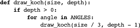
4.3 Fractals in Python ................................. 28

4.3.1 The Koch Snowﬂake........................ 28

4.3.2 Mandelbrot Set ............................ 31

4.4 Online Resources ................................. 33

4.5 Exercises ....................................... 33

5 Introduction to Matplotlib ............................... 35

5.1 Introduction ..................................... 35

5.2 Matplotlib ....................................... 36

5.3 Plot Components .................................. 37

5.4 Matplotlib Architectur e ............................. 38

5.4.1 Backend Layer ............................ 39

5.4.2 The Artist Layer ........................... 40

5.4.3 The Scripting Layer ........................ 41

5.5 Online Resources ................................. 42

6 Graphing with Matplotlib pyplot .......................... 43

6.1 Introduction ..................................... 43

6.2 The pyplot API ................................... 43

6.3 Line Graphs ..................................... 44

6.3.1 Coded Format Strings ....................... 46

6.4 Scatter Graph .................................... 47

6.4.1 When to Use Scatter Graphs .................. 49

6.5 Pie Charts ....................................... 50

6.5.1 Expanding Segments ........................ 52

6.5.2 When to Use Pie Charts ..................... 53

6.6 Bar Charts ...................................... 54

6.6.1 Horizontal Bar Charts ....................... 55

6.6.2 Coloured Bars ............................ 56

6.6.3 Stacked Bar Charts ......................... 57

6.6.4 Grouped Bar Charts ........................ 58

6.7 Figures and Subplots ............................... 60

6.8 3D Graphs ...................................... 63

6.9 Exercises ....................................... 65

7 Graphical User Interfaces ................................ 67

7.1 Introduction ..................................... 67

7.2 GUIs and WIMPS ................................. 68

xiv Contents

7.3 Windowing Frameworks for Python .................... 69

7.3.1 Platform-Independent GUI Libraries ............. 70

7.3.2 Platform-Speciﬁc GUI Libraries ................ 70

7.4 Online Resources ................................. 71

8 The wxPython GUI Library .............................. 73

8.1 The wxPython Library .............................. 73

8.1.1 wxPython Modules ......................... 74

8.1.2 Windows as Objects ........................ 75

8.1.3 A Simple Example ......................... 75

8.2 The wx.App Class ................................. 76

8.3 Window Classes .................................. 78

8.4 Widget/Control Classes ............................. 80

8.5 Dialogs ......................................... 81

8.6 Arranging Widgets Within a Container .................. 82

8.7 Drawing Graphics ................................. 84

8.8 Online Resources ................................. 86

8.9 Exercises ....................................... 86

8.9.1 Simple GUI Application ..................... 86

9 Events in wxPython User Interfaces ........................ 87

9.1 Event Handling ................................... 87

9.2 Event Deﬁnitions ................................. 87

9.3 Types of Events .................................. 88

9.4 Binding an Event to an Event Handler .................. 89

9.5 Implementing Event Handling ........................ 89

9.6 An Interactive wxPython GUI ........................ 92

9.7 Online Resources ................................. 96

9.8 Exercises ....................................... 96

9.8.1 Simple GUI Application ..................... 96

9.8.2 GUI Interface to a Tic Tac Toe Game ........... 98

10 PyDraw wxPython Example Application ..................... 99

10.1 Introduction ..................................... 99

10.2 The PyDraw Application ............................ 99

10.3 The Structure of the Application ...................... 100

10.3.1 Model, View and Controller Architecture ......... 101

10.3.2 PyDraw MVC Architecture ................... 102

10.3.3 Additional Classes ......................... 103

10.3.4 Object Relationships ........................ 104

10.4 The Interactions Between Objects ..................... 105

10.4.1 The PyDrawApp ........................... 105

10.4.2 The PyDrawFrame Constructor ................ 106

Contents xv

10.4.3 Changing the Application Mode ............... 106

10.4.4 Adding a Graphic Object .................... 107

10.5 The Classes ..................................... 108

10.5.1 The PyDrawConstants Class .................. 108

10.5.2 The PyDrawFrame Class ..................... 109

10.5.3 The PyDrawMenuBar Class .................. 110

10.5.4 The PyDrawToolBar Class ................... 111

10.5.5 The PyDrawController Class .................. 111

10.5.6 The DrawingModel Class .................... 113

10.5.7 The DrawingPanel Class ..................... 113

10.5.8 The DrawingController Class .................. 114

10.5.9 The Figure Class .......................... 115

10.5.10 The Square Class .......................... 115

10.5.11 The Circle Class ........................... 116

10.5.12 The Line Class ............................ 116

10.5.13 The Text Class ............................ 117

10.6 References ...................................... 117

10.7 Exercises ....................................... 117

Part II Computer Games

11 Introduction to Games Programming

....................... 121

11.1 Introduction ..................................... 121

11.2 Games Frameworks and Libraries ..................... 121

11.3 Python Games Development ......................... 122

11.4 Using Pygame ................................... 123

11.5 Online Resources ................................. 123

12 Building Games with pygame ............................. 125

12.1 Introduction ..................................... 125

12.2 The Display Surface ............................... 126

12.3 Events ......................................... 127

12.3.1 Event Types .............................. 127

12.3.2 Event Information .......................... 128

12.3.3 The Event Queue .......................... 129

12.4 A First pygame Application .......................... 130

12.5 Further Concepts .................................. 133

12.6 A More Interactive pygame Application ................. 136

12.7 Alternative Approach to Processing Input Devices ......... 138

12.8 pygame Modules .................................. 138

12.9 Online Resources ................................. 139

xvi Contents

13 StarshipMeteors pygame ................................. 141

13.1 Creating a Spaceship Game .......................... 141

13.2 The Main Game Class .............................. 142

13.3 The GameObject Class ............................. 144

13.4 Displaying the Starship ............................. 145

13.5 Moving the Spaceship .............................. 146

13.6 Adding a Meteor Class ............................. 150

13.7 Moving the Meteors ............................... 152

13.8 Identifying a Collision .............................. 152

13.9 Identifying a Win ................................. 154

13.10 Increasing the Number of Meteors ..................... 154

13.11 Pausing the Game ................................. 155

13.12 Displaying the Game Over Message .................... 156

13.13 The StarshipMeteors Game .......................... 157

13.14 Online Resources ................................. 162

13.15 Exercises ....................................... 162

Part III Testing

14 Introduction to Testing .................................. 165

14.1 Introduction ..................................... 165

14.2 Types of Testing .................................. 165

14.3 What Should Be Tested? ............................ 166

14.4 Testing Software Systems ........................... 167

14.4.1 Unit Testing .............................. 168

14.4.2 Integration Testing ......................... 169

14.4.3 System Testing ............................ 169

14.4.4 Installation/Upgrade Testing .................. 170

14.4.5 Smoke Tests .............................. 170

14.5 Automating Testing ................................ 170

14.6 Test Driven Development ........................... 171

14.6.1 The TDD Cycle ........................... 172

14.6.2 Test Complexity ........................... 173

14.6.3 Refactoring ............................... 173

14.7 Design for Testability .............................. 173

14.7.1 Testability Rules of Thumb ................... 173

14.8 Online Resources ................................. 174

14.9 Book Resources .................................. 174

15 PyTest Testing Framework ............................... 175

15.1 Introduction ..................................... 175

15.2 What Is PyTest? .................................. 175

15.3 Setting Up PyTest ................................. 176

15.4 A Simple PyTest Example ........................... 176

Contents xvii

15.5 Working with PyTest .............................. 179

15.6 Parameterised Tests ................................ 183

15.7 Online Resources ................................. 185

15.8 Exercises ....................................... 185

16 Mocking for Testing .................................... 187

16.1 Introduction ..................................... 187

16.2 Why Mock? ..................................... 188

16.3 What Is Mocking? ................................. 190

16.4 Common Mocking Framework Concepts ................ 191

16.5 Mocking Frameworks for Python ...................... 192

16.6 The unittest.mock Library ........................... 192

16.6.1 Mock and Magic Mock Classes ................ 193

16.6.2 The Patchers .............................. 194

16.6.3 Mocking Returned Objects ................... 195

16.6.4 Validating Mocks Have Been Called ............ 196

16.7 Mock and MagicMock Usage ........................ 197

16.7.1 Naming Your Mocks ....................... 197

16.7.2 Mock Classes ............................. 197

16.7.3 Attributes on Mock Classes ................... 198

16.7.4 Mocking Constants ......................... 199

16.7.5 Mocking Properties ......................... 199

16.7.6 Raising Exceptions with Mocks ................ 199

16.7.7 Applying Patch to Every Test Method ........... 200

16.7.8 Using Patch as a Context Manager ............. 200

16.8 Mock Where You Use It ............................ 201

16.9 Patch Order Issues ................................ 201

16.10 How Many Mocks? ................................ 202

16.11 Mocking Considerations ............................ 202

16.12 Online Resources ................................. 203

16.13 Exercises ....................................... 203

Part IV File Input/Output

17 Introduction to Files, Paths and IO......................... 207

17.1 Introduction ..................................... 207

17.2 File Attributes .................................... 209

17.3 Paths .......................................... 211

17.4 File Input/Output .................................. 212

17.5 Sequential Access Versus Random Access ............... 213

17.6 Files and I/O in Python ............................. 214

17.7 Online Resources ................................. 214

xviii Contents

18 Reading and Writing Files ............................... 215

18.1 Introduction ..................................... 215

18.2 Obtaining References to Files ........................ 215

18.3 Reading Files .................................... 217

18.4 File Contents Iteration .............................. 218

18.5 Writing Data to Files ............................... 218

18.6 Using Files and with Statements ...................... 219

18.7 The Fileinput Module .............................. 219

18.8 Renaming Files ................................... 220

18.9 Deleting Files .................................... 220

18.10 Random Access Files .............................. 221

18.11 Directories ...................................... 222

18.12 Temporary Files .................................. 224

18.13 Working with Paths ................................ 225

18.14 Online Resources ................................. 229

18.15 Exercise ........................................ 229

19 Stream IO ............................................ 231

19.1 Introduction ..................................... 231

19.2 What is a Stream? ................................. 231

19.3 Python Streams ................................... 232

19.4 IOBase ......................................... 233

19.5 Raw IO/UnBuffered IO Classes ....................... 234

19.6 Binary IO/Buffered IO Classes ........................ 234

19.7 Text Stream Classes ............................... 236

19.8 Stream Properties ................................. 237

19.9 Closing Streams .................................. 238

19.10 Returning to the open() Function ...................... 238

19.11 Online Resources ................................. 240

19.12 Exercise ........................................ 240

20 Working with CSV Files ................................. 241

20.1 Introduction ..................................... 241

20.2 CSV Files ....................................... 241

20.2.1 The CSV Writer Class ...................... 242

20.2.2 The CSV Reader Class ...................... 243

20.2.3 The CSV DictWriter Class ................... 244

20.2.4 The CSV DictReader Class ................... 245

20.3 Online Resources ................................. 246

20.4 Exercises ....................................... 246

21 Working with Excel Files ................................ 249

21.1 Introduction ..................................... 249

21.2 Excel Files ...................................... 249

Contents xix

21.3 The Openpyxl. Workbook Class ...................... 250

21.4 The Openpyxl. WorkSheet Objects ..................... 250

21.5 Working with Cells ................................ 250

21.6 Sample Excel File Creation Application ................. 251

21.7 Loading a Workbook from an Excel File ................ 253

21.8 Online Resources ................................. 254

21.9 Exercises ....................................... 254

22 Regular Expressions in Python ............................ 257

22.1 Introduction ..................................... 257

22.2 What Are Regular Expressions? ....................... 257

22.3 Regular Expression Patterns .......................... 258

22.3.1 Pattern Metacharacters ...................... 259

22.3.2 Special Sequences .......................... 259

22.3.3 Sets .................................... 260

22.4 The Python re Module ............................. 261

22.5 Working with Python Regular Expressions ............... 261

22.5.1 Using Raw Strings ......................... 261

22.5.2 Simple Example ........................... 262

22.5.3 The Match Object .......................... 262

22.5.4 The search() Function ....................... 263

22.5.5 The match() Function ....................... 264

22.5.6 The Difference Between Matching and Searching ... 265

22.5.7 The ﬁndall() Function ....................... 265

22.5.8 The ﬁnditer() Function ...................... 266

22.5.9 The split() Function ........................ 266

22.5.10 The sub() Function ......................... 267

22.5.11 The compile() Function ...................... 268

22.6 Online Resources ................................. 270

22.7 Exercises ....................................... 270

Part V Database Access

23 Introduction to Databases

................................ 275

23.1 Introduction ..................................... 275

23.2 What Is a Database? ............................... 275

23.2.1 Data Relationships ......................... 276

23.2.2 The Database Schema ....................... 277

23.3 SQL and Databases ................................ 279

23.4 Data Manipulation Language ......................... 280

23.5 Transactions in Databases ........................... 281

23.6 Further Reading .................................. 282

xx Contents

24 Python DB-API ........................................ 283

24.1 Accessing a Database from Python .................... 283

24.2 The DB-API ..................................... 283

24.2.1 The Connect Function ....................... 284

24.2.2 The Connection Object ...................... 284

24.2.3 The Cursor Object ......................... 285

24.2.4 Mappings from Database Types to Python Types ... 286

24.2.5 Generating Errors .......................... 286

24.2.6 Row Descriptions .......................... 287

24.3 Transactions in PyMySQL ........................... 288

24.4 Online Resources ................................. 288

25 PyMySQL Module ..................................... 291

25.1 The PyMySQL Module ............................. 291

25.2 Working with the PyMySQL Module ................... 291

25.2.1 Importing the Module ....................... 292

25.2.2 Connect to the Database ..................... 292

25.2.3 Obtaining the Cursor Object .................. 293

25.2.4 Using the Cursor Object ..................... 293

25.2.5 Obtaining Information About the Results ......... 294

25.2.6 Fetching Results ........................... 294

25.2.7 Close the Connection ....................... 295

25.3 Complete PyMySQL Query Example ................... 295

25.4 Inserting Data to the Database ........................ 296

25.5 Updating Data in the Database ........................ 298

25.6 Deleting Data in the Database ........................ 299

25.7 Creating Tables ................................... 300

25.8 Online Resources ................................. 301

25.9 Exercises ....................................... 301

Part VI Logging

26 Introduction to Logging

................................. 305

26.1 Introduction ..................................... 305

26.2 Why Log? ...................................... 305

26.3 What Is the Purpose of Logging? ...................... 306

26.4 What Should You Log? ............................. 306

26.5 What Not to Log ................................. 307

26.6 Why Not Just Use Print? ............................ 308

26.7 Online Resources ................................. 309

27 Logging in Python...................................... 311

27.1 The Logging Module .............................. 311

27.2 The Logger ...................................... 312

Contents xxi

27.3 Controlling the Amount of Information Logged ........... 313

27.4 Logger Methods .................................. 315

27.5 Default Logger ................................... 316

27.6 Module Level Loggers ............................. 317

27.7 Logger Hierarchy ................................. 318

27.8 Formatters ...................................... 319

27.8.1 Formatting Log Messages .................... 319

27.8.2 Formatting Log Output ...................... 319

27.9 Online Resources ................................. 322

27.10 Exercises ....................................... 322

28 Advanced Logging ..................................... 323

28.1 Introduction ..................................... 323

28.2 Handlers ........................................ 323

28.2.1 Setting the Root Output Handler ............... 325

28.2.2 Programmatically Setting the Handler ........... 326

28.2.3 Multiple Handlers .......................... 328

28.3 Filters .......................................... 329

28.4 Logger Conﬁguration .............................. 330

28.5 Performance Considerations .......................... 333

28.6 Exercises ....................................... 334

Part VII Concurrency and Parallelism

29 Introduction to Concurrency and Parallelism

................. 337

29.1 Introduction ..................................... 337

29.2 Concurrency ..................................... 337

29.3 Parallelism ...................................... 339

29.4 Distribution ...................................... 340

29.5 Grid Computing .................................. 340

29.6 Concurrency and Synchronisation ..................... 342

29.7 Object Orientation and Concurrency .................... 342

29.8 Threads V Processes ............................... 343

29.9 Some Terminology ................................ 344

29.10 Online Resources ................................. 344

30 Threading ............................................ 347

30.1 Introduction ..................................... 347

30.2 Threads ........................................ 347

30.3 Thread States .................................... 347

30.4 Creating a Thread ................................. 348

30.5 Instantiating the Thread Class ........................ 349

30.6 The Thread Class ................................. 350

xxii Contents

30.7 The Threading Module Functions ...................... 352

30.8 Passing Arguments to a Thread ....................... 352

30.9 Extending the Thread Class .......................... 354

30.10 Daemon Threads .................................. 355

30.11 Naming Threads .................................. 356

30.12 Thread Local Data ................................ 357

30.13 Timers ......................................... 358

30.14 The Global Interpreter Lock .......................... 359

30.15 Online Resources ................................. 360

30.16 Exercise ........................................ 360

31 Multiprocessing ........................................ 363

31.1 Introduction ..................................... 363

31.2 The Process Class ................................. 363

31.3 Working with the Process Class ....................... 365

31.4 Alternative Ways to Start a Process .................... 366

31.5 Using a Pool ..................................... 368

31.6 Exchanging Data Between Processes ................... 372

31.7 Sharing State Between Processes ...................... 374

31.7.1 Process Shared Memory ..................... 374

31.8 Online Resources ................................. 375

31.9 Exercises ....................................... 376

32 Inter Thread/Process Synchronisation ....................... 377

32.1 Introduction ..................................... 377

32.2 Using a Barrier ................................... 377

32.3 Event Signalling .................................. 380

32.4 Synchronising Concurrent Code ....................... 382

32.5 Python Locks .................................... 383

32.6 Python Conditions ................................. 386

32.7 Python Semaphores ................................ 388

32.8 The Concurrent Queue Class ......................... 389

32.9 Online Resources ................................. 391

32.10 Exercises ....................................... 391

33 Futures .............................................. 395

33.1 Introduction ..................................... 395

33.2 The Need for a Future .............................. 395

33.3 Futures in Python ................................. 396

33.3.1 Future Creation ............................ 397

33.3.2 Simple Example Future ...................... 397

33.4 Running Multiple Futures ........................... 399

33.4.1 Waiting for All Futures to Complete ............ 400

33.4.2 Processing Results as Completed ............... 402

Contents xxiii

33.5 Processing Future Results Using a Callback .............. 403

33.6 Online Resources ................................. 405

33.7 Exercises ....................................... 405

34 Concurrency with AsyncIO ............................... 407

34.1 Introduction ..................................... 407

34.2 Asynchronous IO ................................. 407

34.3 Async IO Event Loop .............................. 408

34.4 The Async and Await Keywords ...................... 409

34.4.1 Using Async and Await ..................... 409

34.5 Async IO Tasks .................................. 411

34.6 Running Multiple Tasks ............................ 414

34.6.1 Collating Results from Multiple Tasks ........... 414

34.6.2 Handling Task Results as They Are Made

Available ................................ 415

34.7 Online Resources ................................. 416

34.8 Exercises ....................................... 417

Part VIII Reactive Programming

35 Reactive Programming Introduction ........................ 421

35.1 Introduction ..................................... 421

35.2 What Is a Reactive Application? ...................... 421

35.3 The ReactiveX Project .............................. 422

35.4 The Observer Pattern ............................... 422

35.5 Hot and Cold Observables ........................... 423

35.5.1 Cold Observables .......................... 424

35.5.2 Hot Observables ........................... 424

35.5.3 Implications of Hot and Cold Observables ........ 424

35.6 Differences Betw een Event Driven Programming and

Reactive Programming ............................. 425

35.7 Advantages of Reactive Programming .................. 425

35.8 Disadvantages of Reactive Programming ................ 426

35.9 The RxPy Reactive Programming Framework ............. 426

35.10 Online Resources ................................. 426

35.11 Reference ....................................... 427

36 RxPy Observables, Observers and Subjects .................. 429

36.1 Introduction ..................................... 429

36.2 Observables in RxPy ............................... 429

36.3 Observers in RxPy ................................ 430

36.4 Multiple Subscribers/Observers ....................... 432

36.5 Subjects in RxPy ................................. 433

xxiv Contents

36.6 Observer Concurrency .............................. 435

36.6.1 Available Schedulers ........................ 437

36.7 Online Resources ................................. 438

36.8 Exercises ....................................... 438

37 RxPy Operators ....................................... 439

37.1 Introduction ..................................... 439

37.2 Reactive Programming Operators ...................... 439

37.3 Piping Operators .................................. 440

37.4 Creational Operators ............................... 441

37.5 Transformational Operators .......................... 441

37.6 Combinatorial Operators ............................ 443

37.7 Filtering Operators ................................ 444

37.8 Mathematical Operators ............................. 445

37.9 Chaining Operators ................................ 446

37.10 Online Resources ................................. 448

37.11 Exercises ....................................... 448

Part IX Network Programming

38 Introduction to Sockets and Web Services ................... 451

38.1 Introduction ..................................... 451

38.2 Sockets ......................................... 451

38.3 Web Services .................................... 452

38.4 Addressing Services ............................... 452

38.5 Localhost ....................................... 453

38.6 Port Numbers .................................... 454

38.7 IPv4 Versus IPv6 ................................. 455

38.8 Sockets and Web Services in Python ................... 455

38.9 Online Resources ................................. 456

39 Sockets in Python ...................................... 457

39.1 Introduction ..................................... 457

39.2 Socket to Socket Communication ...................... 457

39.3 Setting Up a Connection ............................ 458

39.4 An Example Client Server Application .................. 458

39.4.1 The System Structure ....................... 458

39.4.2 Implementing the Server Application ............ 459

39.5 Socket Types and Domains .......................... 461

39.6 Implementing the Client Application ................... 461

39.7 The Socketserver Module ........................... 463

39.8 HTTP Server .................................... 465

39.9 Online Resources ................................. 469

39.10 Exercises ....................................... 469

Contents xxv

40 Web Services in Python ................................. 471

40.1 Introduction ..................................... 471

40.2 RESTful Services ................................. 471

40.3 A RESTful API .................................. 472

40.4 Python Web Frameworks ............................ 473

40.5 Flask .......................................... 474

40.6 Hello World in Flask ............................... 474

40.6.1 Using JSON .............................. 474

40.6.2 Implementing a Flask Web Service ............. 475

40.6.3 A Simple Service .......................... 475

40.6.4 Providing Routing Information ................ 476

40.6.5 Running the Service ........................ 477

40.6.6 Invoking the Service ........................ 478

40.6.7 The Final Solution ......................... 479

40.7 Online Resources ................................. 479

41 Bookshop Web Service .................................. 481

41.1 Building a Flask Bookshop Service .................... 481

41.2 The Design ...................................... 481

41.3 The Domain Model ................................ 482

41.4 Encoding Books Into JSON .......................... 484

41.5 Setting Up the GET Services ......................... 486

41.6 Deleting a Book .................................. 488

41.7 Adding a New Book ............................... 489

41.8 Updating a Book .................................. 491

41.9 What Happens if We Get It Wrong? ................... 492

41.10 Bookshop Services Listing ........................... 494

41.11 Exercises ....................................... 497

xxvi Contents

Chapter 1

Introduction

1.1 Introduction

I have heard many people over the years say that Python is an easy language to lean

and that Python is also a simple language.

To some extent both of these statements are true; but only to some extent.

While the core of the Python language is easy to lean and relatively simple (in

part thanks to its consistency); the sheer richness of the language constructs and

ﬂexibility available can be overwhelming. In addition the Python environment, its

eco system, the range of libraries available, the often competing options available

etc., can make moving to the next level daunting.

Once you have learned the core elements of the language such as how classes

and inheritance work, how functions work, what are protocols and Abstract Base

Classes etc. Where do you go next?

The aim of this book is to delve into those next steps. The book is organised into

eight different topics:

1. Computer Graphics. The book covers Computer Graphics and Computer

Generated Art in Python as well as Graphical User Interfaces and Graphing/

Charting via MatPlotLib.

2. Games Programming. This topic is covered using the pygam e library.

3. Testing and Mocking. Testing is an important aspect of any software devel-

opment; this book introduces testing in general and the PyTest module in detail.

It also considers mocking within testing including what and when to mock.

4. File Input/Output. The book covers text ﬁle reading and writing as well as

reading and writing CSV and Excel ﬁles. Although not strictly related to ﬁle

input, regulator expressions are incl uded in this section as they can be used to

process textual data held in ﬁles.

5. Database Access. The book introduces databases and relationa l database in

particular. It then presents the Python DB-API database access standard and

J. Hunt, Advanced Guide to Python 3 Programming,

Undergraduate Topics in Computer Science,

https://doi.org/10.1007/978-3-030-25943-3_1

one implementation of this standard, the PyMySQL module used to access a

MySQL database.

6. Logging. An often missed topic is that of logging. The book therefore intro-

duces logging the need for logging, what to log and what not to log as wel l as

the Python logging module.

7. Concurrency and Parallelism. The book provides extensive coverage of

concurrency topics including Threads, Processes and inter thread or process

synchronisation. It also presents Futures and AsyncIO.

8. Reactive Programming. This section of the book introduces Reactive

Programming using the PyRx reactive programming library.

9. Network Programming. The book concludes by introducing socket and web

service communications in Python.

Each section is introduced by a chapter providing the backgro und and key

concepts of that topic. Subsequent chapters then cover various aspects of the topic.

For example, the ﬁrst topic covered is on Computer Graphics. This section has

an introductory chapter on Computer Graphics in general. It then introduces the

Turtle Graphics Python library which can be used to generate a graphical display.

The following chapter considers the subject of Computer Generated Art and uses

the Turtle Graphics library to illustrate these ideas. Thus severa l examples are

presented that might be considered art. The chapter concludes by presenting the

well known Koch Snowﬂake and the Mandelbrot Fractal set.

This is followed by a chapter presenting the MatPlotLib library used for gen-

erating 2D and 3D charts and graphs (such as a line chart, bar chart or scatter

graph).

The section concludes with a chapter on Graphical User Interfaces (or GUIs)

using the wxpython library. This chapter explores what we mean by a GUI and

some of the alternatives available in Python for creating a GUI.

Subsequent topics follow a similar pattern.

Each programming or library oriented chapter also includes numerous sample

programs that can be downloaded from the GutHub repository and executed. These

chapters also include one or more end of chapter exercises (with sample solutions

also in the GutHub repository).

The topics within the book can be read mostly independently of each other. This

allows the reader to dip into subject areas as and when required. For example, the

File Input/Output section and the Database Access section can be read indepen-

dently of each other (although in this case assessing both technologies may be

useful in selecting an appropriate approach to adopt for the long term persistent

storage of data in a particular system).

Within each section there are usually dependencies, for example it is necessary

to understand the pygame library from the ‘Building Games with pygame’

introductory chapter, before exploring the worked case study presented by the

chapter on the StarshipMeteors game. Similarly it is necessary to have read the

Threading and Multiprocessing chapters before reading the Inter Thread/Process

Synchronisation chapter.

2 1 Introduction

Part I

Computer Graphics

Chapter 2

Introduction to Computer Graphics

2.1 Introduction

Computer Graphics are everywhere; they are on your TV, in cinem a adverts, the

core of many ﬁlms, on your tablet or mobile phone and certainly on your PC or Mac

as well as on the dashboard of your car, on your smart watch and in childrens

electronic toys.

However what do we mean by the term Computer Graphics? The term goes back

to a time when many (most) computers were purely textual in terms of their input

and output and very few computers could generate graphical displays let alone

handle input via such a display. However, in terms of this book we take the term

Computer Graphics to include the creation of Graphical User Interfaces (or GUIs),

graphs and charts such as bar charts or line plots of data, graphics in computer

games (such as Space Invaders or Flight Simulator) as well as the generation of 2D

and 3D scenes or images. We also use the term to include Computer Generated Art.

The availability of Computer Graphics is very importan t for the huge acceptance

of computer systems by non computer scientists over the last 40 years. It is in part

thanks to the accessibility of computer systems via computer graphic interfaces that

almost everybody now uses some form of computer system (whether that is a PC, a

tablet, a mobile phone or a smart TV).

A Graphical User Interface (GUI) can capture the essence of an idea or a

situation, often avoiding the need for a long passage of text or textual commands. It

is also because a picture can paint a thousand words; as long as it is the right

picture.

In many situations where the relationships between large amounts of information

must b e conveyed, it is much easier for the user to assimilate this graphically than

textually. Similarly, it is often easier to convey some meaning by manipulating

some system entities on screen, than by combinations of text commands.

For example, a well chosen graph can make clear information that is hard to

determine from a table of the same data. In turn an adventure style game can

J. Hunt, Advanced Guide to Python 3 Programming,

Undergraduate Topics in Computer Science,

https://doi.org/10.1007/978-3-030-25943-3_2

become engaging and immersive with computer graphics which is in marked

contrast to the textual versions of the 1980s. This highlights the advantages of a

visual presentation compared to a purely textual one.

2.2 Background

Every interactive software system has a Human Computer Interface, whether it be a

single text line system or an advanced graphic display. It is the vehicle used by

developers for obtaining information from their user(s), and in turn, every user has

to face some form of computer interface in order to perform any desired computer

operation.

Historically computer systems did not have a Graphical User Interface and rarely

generated a graphical view. These systems from the 60s, 70s and 80s typically

focussed on numerical or data processing tasks. They were accessed via green or

grey screens on a text oriented terminal. There was little or no opportunity for

graphical output.

However, during this period various researchers at laboratories such as Stanford,

MIT, Bell Telephone Labs and Xerox were looking at the possibilities that graphic

systems might offer to computers. Indeed even as far back as 1963 Ivan Sutherland

showed that interactive computer graphics were feasible with his Ph.D. thesis on the

Sketchpad system.

2.3 The Graphical Computer Era

Graphical computer displays and interactive graphical interfaces became a common

means of human–computer interaction during the 1980s. Such interfaces can save a

user from the need to learn complex commands. They are less likely to intimidate

computer naives and can provide a large amount of information quickly in a form

which can be easily assimilated by the user.

The widespread use of high quality graphical interfaces (such as those provided

by the Apple Macintosh and the early Windows interface) led many computer users

to expect such interfaces to any software they use. Indeed these systems paved the

way for the type of interface that is now omnipresent on PCs, Macs, Linux boxes,

tablets and smart phones etc. This graphical user interface is based on the WIMP

paradigm (Windows, Icons, Menus and Pointers) which is now the prevalent type

of graphical user interface in use today.

The main advantage of any window-based system, an d particularly of a WIMP

environment, is that it requires only a small amount of user training. There is no

need to learn complex commands, as most operations are available either as icons,

operations on icons, user actions (such as swiping) or from menu options, and are

easy to use. (An icon is a small graphic object that is usual ly symbolic of an

6 2 Introduction to Computer Graphics

operation or of a larger entity such as an application program or a ﬁle). In general,

WIMP based systems are simple to learn, intuitive to use, easy to retain and

straightforward to work with.

These WIMP systems are exempliﬁed by the Appl e Macintosh interface (see

Goldberg and Robson as well as Tesler), which was inﬂuenced by the pioneering

work done at the Palo Alto Research Center on the Xerox Star Machine. It was,

however, the Macintosh which brought such interfaces to the mass market, and ﬁrst

gained acceptance for them as tools for business, home and industry. This interface

transformed the way in which humans expected to interact with their computers,

becoming a de facto standard, which forced other manufacturers to provide similar

interfaces on their own machines, for example Microsoft Windows for the PC.

This type of interface can be augmented by providing direct manipulation

graphics. These are graphics which can be grabbed and manipulated by the user,

using a mouse, to perform some operation or action. Icons are a simple version of

this, the “opening” of an icon causes either the associated application to execute or

the associated window to be displayed.

2.4 Interactive and Non Interactive Graphics

Computer graphics can be broadly subdivided into two categories:

• Non Interactive Computer Graphics

• Interactive Computer Graphics.

In Non Interactive Computer Graphics (aka Passive Computer Graphics) an

image is generated by a computer typically on a computer screen; this image can be

viewed by the u ser (however they cannot interact with the image). Examples of

non-interactive graphics presented later in this book include Computer Generated

Art in which an image is generated using the Python Turtle Graphics library. Such

an image can viewed by the user but not modiﬁed. Another example might be a

basic bar chart generated using MatPlotLib which presents some set of data.

Interactive Computer Graphics by contrast, involve the user interacting with the

image displayed in the screen in some way, this might be to modify the data being

displayed or to change they way in which the image is being rendered etc. It is

typiﬁed by interactive Graphical User Interfaces (GUIs) in which a user interacts with

menus, buttons, input ﬁeld, sliders, scrollbars etc. However, other visual displays can

also be interactive. For example, a slider could be used with a MatplotLib chart. This

display could present the number of sales made on a particular date; as the slider is

moved so the data changes and the chart is modiﬁed to show different data sets.

Another example is represented by all computer games which are inherently

interactive and most, if not all, update their visual display in response to some user

inputs. For example in the classic ﬂight simulator game, as the user moves the

joystick or mouse, the simulated plane moves accordingly and the display presented

to the user updates.

2.3 The Graphical Computer Era 7

2.5 Pixels

A key concept for all computer graphics systems is the pixel. Pixel was originally a

word formed from combining and shortening the words picture (or pix) and ele-

ment. A pixel is a cell on the computer screen. Each cell represents a dot on the

screen. The size of this dot or cell and the number of cells available will vary

depending upon the type, size and resolution of the screen. For example, it was

common for early Windows PCs to have a 640 by 480 resolution display (using a

VGA graphics card). This relates to the number of pixels in terms of the width and

height. This meant that there were 640 pixels across the screen with 480 rows of

pixels down the screen. By contrast todays 4K TV displays have 4096 by 2160

pixels.

The size and number of pixels available affects the quality of the image as

presented to a user. With lower resolution displays (with fewer indi vidual pixels)

the image may appear blocky or poorly deﬁned; where as with a higher resolution it

may appear sharp and clear.

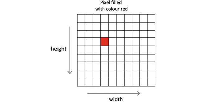
Each pixel ca n be referenced by its locat ion in the display grid. By ﬁlling a

pixels on the screen with different colours various images/displays can be created.

For example, in the following picture a single pixel has been ﬁlled at position 4

by 4:

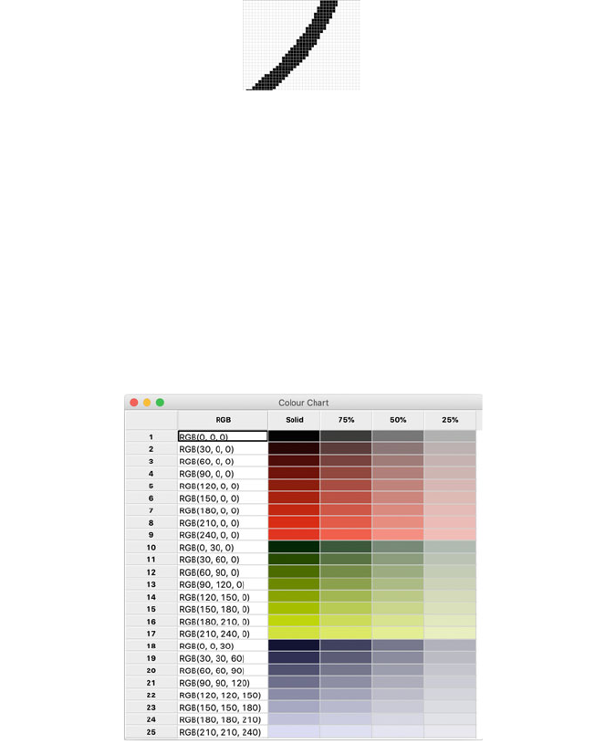
A sequence of pixels can form a line, a circle or any number of different shapes.

However, since the grid of pixels is based on individual points, a diagonal line or a

circle may need to utilise multiple pixels which when zoomed may have jagged

edges. For example, the following picture shows part of a circle on which we have

zoomed in:

8 2 Introduction to Computer Graphics

Each pixel can have a colour and a transparency associated with it. The range of

colours available depends on the display system being used. For example, mono

chrome displays only allow black and white, where as a grey scale display only

allows various shades of grey to be displayed. On modern systems it is usually

possible to represent a wide range of colours using the tradition RGB colour codes

(where R represents Red, G represents Green and B represents Blue). In this

encoding solid Red is represented by a code such as [255, 0, 0] where as solid

Green is represented by [0, 255, 0] and solid Blue by [0, 0, 255]. Based on this idea

various shades can be represented by combination of these codes such as Orange

which might be represented by [255, 150, 50]. This is illustrated below for a set of

RGB colours using different red, green and blue values :

In addition it is possible to apply a transparency to a pixel. This is used to

indicate how solid the ﬁll colour should be. The above grid illustrates the effect of

applying a 75%, 50% and 25% transparency to colours displayed using the Python

wxPython GUI library. In this library the transparency is referred to as the alpha

opaque value. It can have values in the range 0–255 where 0 is completely trans-

parent and 255 is completely solid.

2.5 Pixels 9

2.6 Bit Map Versus Vector Graphics

There are two ways of generating an image/display across the pixels on the screen.

One approach is known as bit mapped (or raster) graphics and the other is known as

vector graphics. In the bit mapped approach each pixel is mapped to the values to

be displayed to create the image. In the vector graphics approach geometric shapes

are described (such as lines and points) and these are then rendered onto a display.

Raster graphics are simpler but vector graphics provide much more ﬂexibility and

scalability.

2.7 Buffering

One issue for interactive graphical displays is the ability to change the display as

smoothly and cleanly as possible. If a display is jerky or seems to jump from one

image to another, then users will ﬁnd it uncomfortable. It is therefore common to

drawn the next display on some in memory structure; often referred to as a buffer.

This buffer can then be rendered on the display once the whole image has been

created. For example Turtle Graphics allows the user to deﬁne how many changes

should be made to the display before it is rendered (or drawn) on to the screen. This

can signiﬁcantly speed up the performance of a graphic application.

In some cases systems will use two buffers; often referred to as double buffering.

In this approach one buffer is being render ed or drawn onto the screen while the

other buffer is being updated. This can signiﬁcantly improve the overall perfor-

mance of the system as modern computers can perform calculations and generate

data much faster than it can typically be drawn onto a screen.

2.8 Python and Computer Graphics

In the remainder of this section of the book we will look at generating computer

graphics using the Python Turtle Graphics library. We will also discuss using this

library to create Computer Generated Art. Following this we will explore the

MatPlotLib library used to generate charts and data plots such as bar charts, scatter

graphs, line plots and heat maps etc. We will then explore the use of Python

libraries to create GUIs using menus, ﬁelds, tables etc.

10 2 Introduction to Computer Graphics

2.9 References

The following are referenced in this chapter:

• I.E. Sutherland, Sketchpad: a man-machine graphical communication system

(courtesy Computer Laboratory, University of Cambridge UCAM-CL-TR-574,

September 2003), January 1963.

• D.C. Smith, C. Irby, R. Kimball, B. Verplank, E. Harslem, Designing the Star

user interface. BYTE 7(4), 242–282 (1982).

2.10 Online Resources

The following provide further reading material:

•

https://en.wikipedia.org/wiki/Sketchpad Ivan Sutherlands Sketchpad from 1963.

•

http://images.designworldonline.com.s3.amazonaws.com/CADhistory/

Sketchpad_A_Man-Machine_Graphical_Communication_System_Jan63.pdf

Ivan Sutherlands Ph.D. 1963.

•

https://en.wikipedia.org/wiki/Xerox_Star The Xerox Star compu ter and GUI.

2.9 References 11

Chapter 3

Python Turtle Graphics

3.1 Introduction

Python is very well supported in terms of graphics libraries. One of the most widely

used graphics libraries is the Turtle Graphics library introduced in this chapter. This

is partly because it is straight forward to use and partly because it is provided by

default with the Python environment (and this you do not need to install any

additional libraries to use it).

The chapter concludes by brieﬂy considering a number of other graphic libraries

including PyOpen GL. The PyOpenGL library can be used to create sophisticated

3D scenes.

3.2 The Turtle Graphics Library

3.2.1 The Turtle Module

This provides a library of features that allow what are known as vector graphics to

be created. Vector graphics refers to the lines (or vectors) that can be drawn on the

screen. The drawing area is often referred to as a drawing plane or drawing board

and has the idea of x, y coordinates.

The Turtle Graphics library is intended just as a basic drawing tool; other

libraries can be used for drawing two and three dimensional graphs (such as

MatPlotLib) but those tend to focus on speciﬁc types of graphical displays.

The idea behind the Turtle module (and its name) derives from the Logo pro-

gramming language from the 60s and 70s that was designed to introduce program-

ming to children. It had an on screen turtle that could be controlled by commands such

as forward (which would move the turtle forward), right (which would turn the turtle

by a certain number of degrees), left (which turns the turtle left by a certain number of

J. Hunt, Advanced Guide to Python 3 Programming,

Undergraduate Topics in Computer Science,

https://doi.org/10.1007/978-3-030-25943-3_3

degrees) etc. This idea has continued into the current Python Turtle Graphics library

where commands such as turtle.forward(10) moves the turtle (or cursor as it

is now) forward 10 pixels etc. By combining together these apparently simple

commands, it is possible to create intricate and quiet complex shapes.

3.2.2 Basic Turtle Graphics

Although the turtle module is built into Python 3 it is necessary to import the

module before you use it:

There are in fact two ways of working with the turtle module; one is to use

the classes available with the library and the other is to use a simpler set of functions

that hide the classes and objects. In this chapter we will focus on the set of functions

you can use to create drawings with the Turtle Graphics library.

The ﬁrst thing we will do is to set up the window we will use for our drawings;

the TurtleScreen class is the parent of all screen implementations used for

whatever operating system you are running on.

If you are using the functions provided by the turtle module, then the screen

object is initialised as appropriate for your operating system. This means that you

can just focus on the following functions to conﬁgure the layout/display such as this

screen can have a title, a size, a starting location etc.

The key functions are:

• setup(width, height, startx, starty) Sets the size and position of

the main window/screen. The parameters are:

– width—if an integer, a size in pixels, if a ﬂoat, a fraction of the screen;

default is 50% of screen.

– height—if an integer, the height in pixels, if a ﬂoat, a fraction of the

screen; default is 75% of screen.

– startx—if positive, starting position in pixels from the left edge of the

screen, if negative from the right edge, if None, center window horizontally.

– starty—if positive, starting position in pixels from the top edge of the

screen, if negative from the bottom edge, if None, center window vertically.

• title(titles tring) sets the title of the screen/window.

• exitonclick( ) shuts down the turtle graphics screen/window when the use

clicks on the screen.

• bye() shuts down the turtle graphics screen/window.

• done() starts the main event loop; this must be the last statement in a turtle

graphics program.

import turtle

14 3 Python Turtle Graphics

• speed(speed) the drawing speed to use, the default is 3. The higher the

value the faster the drawing takes place, values in the range 0–10 are accepted.

• turtle.trace r(n = None) This can be used to batch updates to the turtle

graphics screen. It is very useful when a drawing become large and complex. By

setting the number (n) to a large number (say 600) then 600 elements will be

drawn in memory before the actual screen is updated in one go; this can sig-

niﬁcantly speed up the generation of for example, a fractal picture. When called

without arguments, returns the currently stor ed value of n.

• turtle.updat e() Perform an update of the turtle screen; this should be

called at the end of a program when tracer() has been used as it will ensure

that all elements have been drawn even if the tracer threshold has not yet been

reached.

• pencolor(col or) used to set the colour used to draw lines on the screen;

the color can be speciﬁed in numerous ways including using named colours set

as ‘red’, ‘blue’, ‘green’ or using the RGB colour codes or by specifying the

color using hexadecimal numbers. For more information on the named colours

and RGB colour codes to use see

https://www.tcl.tk/man/tcl/TkCmd/colors.htm.

Note all colour methods use American spellings for example this method is

pencolor (not pencolour).

• ﬁllcolor(color) used to set the colour to use to ﬁll in closed areas within

drawn lines. Again note the spelling of colour!

The following code snippet illustrates some of these functions:

We can now look at how to actually draw a shape onto the screen.

The cursor on the screen has several properties; these include the cu rrent

drawing colour of the pen that the cursor moves, but also its current position (in the

x, y coordinates of the screen) and the direction it is currently facing. We have

import turtle

# set a title for your canvas window

turtle.title('My Turtle Animation')

# set up the screen size (in pixels)

# set the starting point of the turtle (0, 0)

turtle.setup(width=200, height=200, startx=0, starty=0)

# sets the pen color to red

turtle.pencolor('red')

# …

# Add this so that the window will close when clicked on

turtle.exitonclick()

3.2 The Turtle Graphics Library 15

already seen that you can control one of these properties using the pencolor()

method, other methods are used to control the cursor (or turtle) and are presented

below.

The direction in which the cursor is pointing can be altered using several

functions including:

• right(angle) Turn cursor right by angle units.

• left(angle) Turn the cursor left by angle units.

• setheading(t o_angle) Set the orientation of the cursor to to_angle.

Where 0 is east, 90 is north, 180 is west and 270 is south.

You can move the cursor (and if the pen is down this will draw a line) using:

• forward(dist ance) move the cursor forward by the speciﬁed distance in

the direction that the cursor is currently pointing. If the pen is down then draw a

line.

• backward(dis tance) move the cursor backward by distance in the

opposite direction that in which the cursor is pointing.

And you can also explicitly position the cursor:

• goto(x, y) move the cursor to the x, y location on the screen speciﬁed; if the

pen is down draw a line. You can also use steps and set position to do the same

thing.

• setx(x) sets the cursor’s x coordinate, leaves the y coordinate unchanged.

• sety(y) sets the cursor’s y coordinate, leaves the x coordinate unchanged.

It is also possible to move the cursor without drawing by modifying whether the

pen is up or down:

• penup() move the pen up—moving the cursor will no longer draw a line.

• pendown() move the pen down—moving the cursor will now draw a line in

the current pen colour.

The size of the pen can also be controlled:

• pensize(widt h) set the line thickness to width. The method width() is

an alias for this method.

It is also possible to draw a circle or a dot:

• circle(radiu s, extent, steps) draws a circle using the given radius.

The extent determines how much of the circle is drawn; if the extent is not given

then the whole circle is drawn. Steps indicates the number of steps to be used to

drawn the circle (it can be used to draw regular polygons).

• dot(size, color) draws a ﬁlled circle with the diameter of size using the

speciﬁed color.

16 3 Python Turtle Graphics

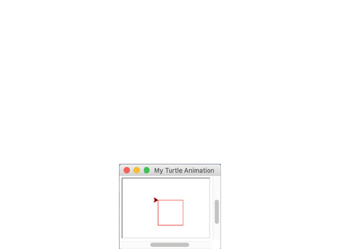
You can now use some of the above methods to draw a shape on the screen. For

this ﬁrst example, we will keep it very simple, we will draw a simple square:

The above moves the cursor forward 50 pixels then turns 90° before repeating

these steps three times. The end result is that a square of 50  50 pixels is drawn on

the screen:

Note that the cursor is displayed during drawing (this can be turned off with

turtle.hideturtle() as the cursor was originally referred to as the turtle).

3.2.3 Drawing Shapes

Of course you do not need to just use ﬁxed values for the shapes you draw, you can

use variables or calculate positions based on expressions etc.

For example, the following program creates a sequences of squares rotated

around a central location to create an engaging image:

# Draw a square

turtle.forward(50)

turtle.right(90)

turtle.forward(50)

turtle.right(90)

turtle.forward(50)

turtle.right(90)

turtle.forward(50)

turtle.right(90)

3.2 The Turtle Graphics Library 17

In this program two functions have been deﬁned, one to setup the screen or

window with a title and a size and to turn off the cursor display. The second

function takes a size parameter and uses that to draw a square. The main part of the

program then sets up the window and uses a for loop to draw 12 squares o f 50

pixels each by continuously rotat ing 120° between each square. Note that as we do

not need to reference the loop variable we are using the ‘_’ format which is

considered an anonymous loop variable in Python.

The image generated by this program is shown below:

import turtle

def setup():

""" Provide the config for the screen """

turtle.title('Multiple Squares Animation')

turtle.setup(100, 100, 0, 0)

turtle.hideturtle()

def draw_square(size):

""" Draw a square in the current direction """

turtle.forward(size)

turtle.right(90)

turtle.forward(size)

turtle.right(90)

turtle.forward(size)

turtle.right(90)

turtle.forward(size)

setup()

for _ in range(0, 12):

draw_square(50)

# Rotate the starting direction

turtle.right(120)

# Add this so that the window will close when clicked o

turtle.exitonclick()

18 3 Python Turtle Graphics

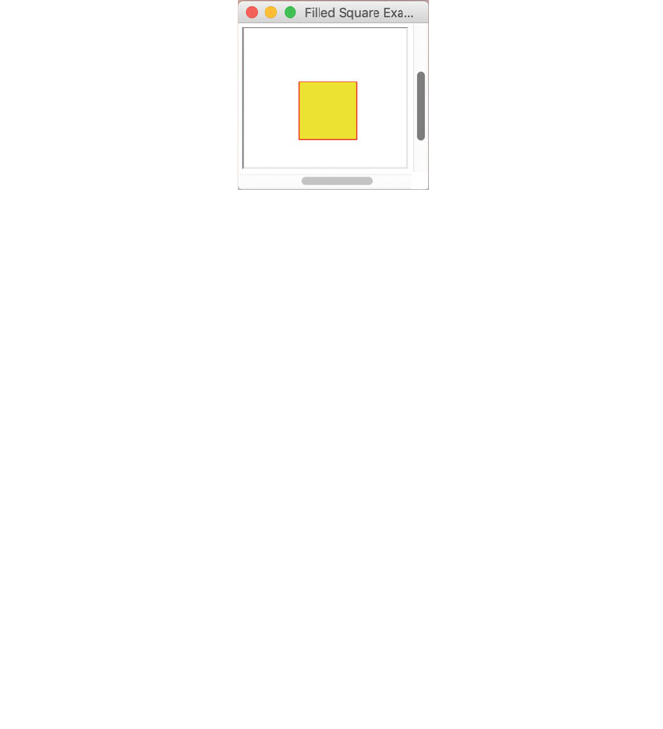
3.2.4 Filling Shapes

It is also possible to ﬁll in the area within a drawn shape. For example, you might

wish to ﬁll in one of the squares we have drawn as shown below:

To do this we can use the begin_ﬁll() and end_ﬁll() functions:

• begin_ﬁll() indicates that shapes should be ﬁlled with the current ﬁll col-

our, this function should be called just before drawing the shape to be ﬁlled.

• end_ﬁll() called after the shape to be ﬁlled has been ﬁnished. This will cause

the shape drawn since the last call to begin_ﬁll() to be ﬁlled using the

current ﬁll colour.

• ﬁlling() Return the current ﬁll state (True if ﬁlling, False if not).

The following program uses this (and the earlier draw_square() function) to

draw the above ﬁlled square:

3.3 Other Graphics Libraries

Of course Turtle Graphics is not the only graphics option available for Python;

however other graphi cs libraries do not come pre-packed with Python and must be

downloaded using a tool such as Anaconda, PIP or PyCharm.

turtle.title('Filled Square Example')

turtle.setup(100, 100, 0, 0)

turtle.hideturtle()

turtle.pencolor('red')

turtle.fillcolor('yellow')

turtle.begin_fill()

draw_square(60)

turtle.end_fill()

turtle.done()

3.2 The Turtle Graphics Library 19

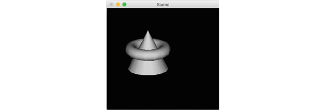
• PyQtGraph. The PyQtGraph library is pure Python library oriented towards

mathematics, scientiﬁc and engineering graphic app lications as well as GUI

applications. For more information see

http://www.pyqtgraph.org.

• Pillow. Pillow is a Python imaging library (based on PIL the Python Imaging

library) that provides image processing capabilities for use in Python. For more

information on Pillow see

https://pillow.readthedocs.io/en/stable.

• Pyglet. pyglet is anothe r windowing and multimedia library for Python. See

https://bitbucket.org/pyglet/pyglet/wiki/Home.

3.4 3D Graphics

Although it is certainly possible for a developer to create convincing 3D images

using Turtle Graphics; it is not the primary aim of the library. This means that there

is no direct support for creating 3D images other than the basic cursor moving

facilities and the programers skill.

However, there are 3D graphics libraries available for Python. One such library is

Panda3D (

https://www.pand a3d.org) while another is VPython (https://vpython.org)

while a third is pi3d (

https://pypi.org/project/pi3d). However we will brieﬂy look at

the PyOpenGL library as this builds on the very widely used OpenGL library.

3.4.1 PyOpenGL

PyOpenGL his an open source project that provides a set of bindings (or wrappings

around) the OpenGL library. OpenGL is the Open Graphics Library which is a

cross language, cross platform API for rendering 2D and 3D vector graphics.

OpenGL is used in a wide range of applications from games, to virtual reality,

through data and information visualisation systems to Computer Aided Design

(CAD) systems. PyOpenGL provides a set of Python functions that call out from

Python to the underlying OpenGL libraries. This makes it very easy to create 3D

vector based images in Python using the industry standard OpenGL library. A very

simple examples of an image created using PyOpenGL is given below:

20 3 Python Turtle Graphics

3.5 Online Resources

The following provide further reading material:

•

https://docs.python.org/3/library/turtle.html Turtle graphics documentation.

•

http://pythonturtle.org/ The Python Turtle programming environment—this

intended for teaching the basic concepts behind programming using the Turtle

graphics library.

•

http://pyopengl.sourceforge.net The PyOpenGL home page.

•

https://www.opengl.org The Open GL home page.

3.6 Exercises

The aim of this exercise is to create a graphic display using Python Turtle Graphics.

You should create a simple program to draw an octagon on the Turtle Graphics

screen.

Modify your program so that there is an hexagon drawing function. This

function should take three parameters, the x, and y coordinates to start drawing the

octagon and the size of each side of the octagon.

Modify your program to draw the hexagon in multiple locations to create the

following picture:

3.5 Online Resources 21

Chapter 4

Computer Generated Art

4.1 Creating Computer Art

Computer Art is deﬁned as any art that uses a computer. However, in the context of

this book we mean it to be art that is generated by a computer or more speciﬁcally a

computer program. The following example, illustrates how in a very few lines of

Python code, using the Turtle graphics library, you can create images that might be

considered to be computer art.

The following image is generated by a recursive function that draws a circle at a

given x, y location of a speciﬁed size. This function recursively calls itself by

modifying the parameters so that smaller and smaller circles are drawn at different

locations until the size of the circles goes below 20 pixels.

J. Hunt, Advanced Guide to Python 3 Programming,

Undergraduate Topics in Computer Science,

https://doi.org/10.1007/978-3-030-25943-3_4

The program used to generate this picture is given below for reference:

import turtle

WIDTH = 640

HEIGHT = 360

def setup_window():

# Set up the window

turtle.title('Circles in My Mind')

turtle.setup(WIDTH, HEIGHT, 0, 0)

turtle.colormode(255)

# Indicates RGB numbers will be in

the range 0 to 255

turtle.hideturtle()

# Batch drawing to the screen for faster rendering

turtle.tracer(2000)

# Speed up drawing process

turtle.speed(10)

turtle.penup()

def draw_circle(x, y, radius, red=50, green=255, blue=10,

width=7):

""" Draw a circle at a specific x, y location.

Then draw four smaller circles recursively"""

colour = (red, green, blue)

# Recursively drawn smaller circles

if radius > 50:

# Calculate colours and line width for smaller circles

if red < 216:

red = red + 33

green = green - 42

blue = blue + 10

width -= 1

24 4 Computer Generated Art

# Run the program

print('Starting')

setup_window()

draw_circle(25, -100, 200)

# Ensure that all the drawing is rendere

turtle.update()

print('Done')

turtle.done()

There are a few points to note about this program. It uses recursion to draw the

circles with smaller and smaller circles being drawn until the radius of the circles

falls below a certain threshold (the termination point ).

It also uses the turtle.tracer() function to speed up drawing the picture

as 2000 changes will be buffered before the screen is updated.

Finally, the colours used for the circles are changed at each level of recession; a

very simple approach is used so that the Red, Green and Blue codes are changed

resulting in different colour circles. Also a line width is used to reduce the size of

the circle outline to add more interest to the image.

4.2 A Computer Art Generator

As another example of how you can use Turtle graphics to create computer art, the

following program randomly generates RGB colours to use for the lines being

drawn which gives the pictures more interest. It also allows the user to input an

else:

red = 0

green = 255

# Calculate the radius for the smaller circles

new_radius = int(radius / 1.3)

# Drawn four circles

draw_circle(int(x + new_radius), y, new_radius, red,

green, blue, width)

draw_circle(x - new_radius, y, new_radius, red, green,

blue, width)

draw_circle(x, int(y + new_radius), new_radius, red,

green, blue, width)

draw_circle(x, int(y - new_radius), new_radius, red,

green, blue, width)

# Draw the original circle

turtle.goto(x, y)

turtle.color(colour)

turtle.width(width)

turtle.pendown()

turtle.circle(radius)

turtle.penup()

4.1 Creating Computer Art 25

angle to use when changing the direction in which the line is drawn. As the drawing

happens within a loop even this simple change to the angle used to draw the lines

can generate very different pict ures.

# Lets play with some colours

import turtle

from random import randint

def get_input_angle():

""" Obtain input from user and convert to an int"""

message = 'Please provide an angle:'

value_as_string = input(message)

while not value_as_string.isnumeric():

print('The input must be an integer!')

value_as_string = input(message)

return int(value_as_string)

def generate_random_colour():

"""Generates an R,G,B values randomly in range

0 to 255 """

r = randint(0, 255)

g = randint(0, 255)

b = randint(0, 255)

return r, g, b

print('Set up Screen')

turtle.title('Colourful pattern')

turtle.setup(640, 600)

turtle.hideturtle()

turtle.bgcolor('black')

# Set the background colour of the

screen

turtle.colormode(255) # Indicates RGB numbers will be in the

range 0 to 255

turtle.speed(10)

angle = get_input_angle()

print('Start the drawing')

for i in range(0, 200):

turtle.color(generate_random_colour())

turtle.forward(i)

turtle.right(angle)

print('Done')

turtle.done()

26 4 Computer Generated Art

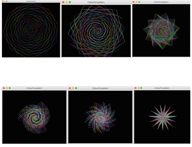
Some sample images generated from this program are given below. The left

most picture is generated by inputting an angle of 38 degrees, the picture on the

right uses an angle of 68 degrees and the bottom picture an angle of 98 degrees.

The following pictures below use angles of 118, 138 and 168 degrees respectively.

What is interesting about these images is how different each is; even though they

use exactly the same program. This illustrates how algorithmic or computer gen-

erated art can be as subtle and ﬂexible as any other art form. It also illustrates that

even with such a process it is still up to the human to determine which image (if

any) is the most aesthetically pleasing.

4.2 A Computer Art Generator 27

4.3 Fractals in Python

Within the arena of Computer Art fractals are a very well known art form. Factrals

are recurring patterns that are calcul ated either using an iterative approach (such as

a for loop) or a recursive approach (when a function calls itself but with modi ﬁed

parameters). One of the really interesting features of fractals is that they exhibit the

same pattern (or nearly the same pattern) at successive levels of granularity. That is,

if you magniﬁed a fractal image you would ﬁnd that the same pattern is being

repeated at successively smaller and smaller magniﬁcations. This is known as ex-

panding symmetry or unfolding symmetry; if this replication is exactly the same at

every scale, then it is called afﬁne self-similar.

Fractals have their roots in the world of mathematics starting in the 17th century,

with the term fractal being coined in the 20th century by mathematical Benoit

Mandelbrot in 1975. One often cited description that Mandelbrot published to

describe geometric fractals is

a rough or fragmented geometric shape that can be split into parts, each of which is (at least

approximately) a reduced-size copy of the whole.

For more information see Mandelbrot, Benoît B. (1983). The fractal geometry of

nature. Macmillan. ISBN (978-0-7167-1186-5).

Since the later part of the 20th century fractals have been a commonly used way

of creating computer art.

One example of a fractal often used in computer art is the Koch snow ﬂake, while

another is the Mandelbrot set. Both of these are used in this chapter as examples to

illustrate how Python and the Turtle graphics library can be used to create fractal

based art.

4.3.1 The Koch Snowﬂake

The Koch snowﬂake is a fractal that begins with equilateral triangle and then

replaces the middle third of every line segment with a pair of line segments that

form an equilateral bump. This replacement can be performed to any depth gen-

erating ﬁner and ﬁner grained (smaller and smaller) triangles until the overall shape

resembles a snow ﬂake.

28 4 Computer Generated Art

The following program can be used to generate a Koch snowﬂake with different

levels of recursion. The larger the number of levels of recursion the more times each

line segment is dissected.

import turtle

# Set up Constants

ANGLES = [60, -120, 60, 0]

SIZE_OF_SNOWFLAKE = 300

def get_input_depth():

""" Obtain input from user and convert to an int"""

message = 'Please provide the depth (0 or a positive

interger):'

value_as_string = input(message)

while not value_as_string.isnumeric():

print('The input must be an integer!')

value_as_string = input(message)

return int(value_as_string)

def setup_screen(title, background='white', screen_size_x=640,

screen_size_y=320, tracer_size=800):

print('Set up Screen')

turtle.title(title)

turtle.setup(screen_size_x, screen_size_y)

turtle.hideturtle()

turtle.penup()

turtle.backward(240)

# Batch drawing to the screen for faster rendering

turtle.tracer(tracer_size)

turtle.bgcolor(background)

# Set the background colour of

the screen

4.3 Fractals in Python 29

Several different runs of the program are shown below with the depth set at 0, 1,

3 and 7.

def draw_koch(size, depth):

if depth > 0:

for angle in ANGLES:

draw_koch(size / 3, depth - 1)

turtle.left(angle)

else:

turtle.forward(size)

depth = get_input_depth()

setup_screen('Koch Snowflake (depth ' + str(depth) + ')',

background='black',

screen_size_x=420, screen_size_y=420)

# Set foreground colours

turtle.color('sky blue')

# Ensure snowflake is centred

turtle.penup()

turtle.setposition(-180,0)

turtle.left(30)

turtle.pendown()

# Draw three sides of snowflake

for _ in range(3):

draw_koch(SIZE_OF_SNOWFLAKE, depth)

turtle.right(120)

# Ensure that all the drawing is rendered

turtle.update()

print('Done')

turtle.done()

30 4 Computer Generated Art

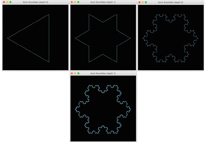
Running the simple draw_koch() function with different depths makes it easy

to see the way in which each side of a triangle can be dissected into a further

triangle like shape. This can be repeated to multiple depths giving a more detailed

structured in which the same shape is repeated again and again.

4.3.2 Mandelbrot Set

Probably one of the most famous fractal images is based on the Mandelbrot set.

The Mandelbrot set is the set of complex numbers c for which the function z*

z+c does not diverge when iterated from z = 0 for which the sequence of

functions (func(0), func(func(0)) etc.) remains bounded by an absolute value. The

deﬁnition of the Mandelbrot set and its name is down to the French

mathematician Adrien Douady, who named it as a tribute to the mathematician

Benoit Mandelbrot.

Mandelbrot set images may be created by sampling the complex numbers and

testing, for each sample point c, whether the sequence func(0), func(func(0)) etc.

ranges to inﬁnity (in practice this means that a test is made to see if it leaves some

predetermined bounded neighbourhood of 0 after a predetermined number of

iterations). Treating the real and ima ginary parts of c as image coordinates on

the complex plane, pixels may then be coloured according to how soon the

sequence crosses an arbitrarily chosen threshold, with a special color (usually

black) used for the values of c for which the sequence has not crossed the threshold

4.3 Fractals in Python 31

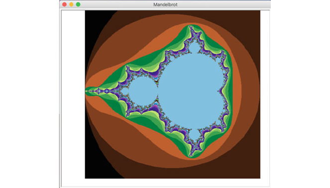
after the predetermined number of iterations (this is necessary to clearly distinguish

the Mandelbrot set image from the image of its complement).

The following image was generated for the Mandelbrot set using Python and

Turtle graphics.

The program used to generate this image is given below:

for y in range(IMAGE_SIZE_Y):

zy = y * (MAX_Y - MIN_Y) / (IMAGE_SIZE_Y - 1) + MIN_Y

for x in range(IMAGE_SIZE_X):

zx = x * (MAX_X - MIN_X) / (IMAGE_SIZE_Y - 1) + MIN_X

z = zx + zy * 1j

c = z

for i in range(MAX_ITERATIONS):

if abs(z) > 2.0:

break

z = z * z + c

turtle.color((i % 4 * 64, i % 8 * 32, i % 16 * 16))

turtle.setposition(x - SCREEN_OFFSET_X,

y - SCREEN_OFFSET_Y)

turtle.pendown()

turtle.dot(1)

turtle.penup()

32 4 Computer Generated Art

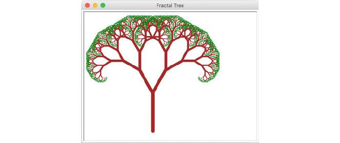
4.4 Online Resources

The following provide further reading material:

•

https://en.wikipedia.org/wiki/Fractal For the Wikipedia page on Fractals.

•

https://en.wikipedia.org/wiki/Koch_snow ake The Wikipedia page on the Koch

snowﬂake.

•

https://en.wikipedia.org/wiki/Mandelbrot_set Wikipedia page on the Mandel-

brot set.

4.5 Exercises

The aim of this exercise is to create a Fractal Tree.

A Fractal Tree is a tree in which the overall structure is replicated at ﬁner and

ﬁner levels through the tree until a set of leaf elements are reached.

To draw the fractal tree you will need to:

• Draw the trunk.

• At the end of the trunk, split the trunk in two with the left trunk and the right

trunk being 30° left/right of the original trunk. For aesth etic purposes the trunk

may become thinner each time it is split. The trunk may be drawn in a particular

colour such as brown.

• Continue this until a maximum number of splits have occurred (or the trunk size

reduces to a particular minimum). You have now reached the leaves (you may

draw the leaves in a different colour e.g. green).

An example of a Fractal Tree is given below:

4.4 Online Resources 33

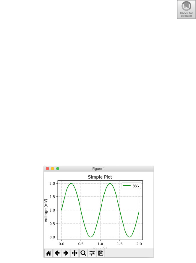
Chapter 5

Introduction to Matplotlib

5.1 Introduction

Matplotlib is a Python graphing and plotting library that can generate a variety of

different types of graph or chart in a variety of different formats. It can be used to

generate line charts, scatter graphs, heat maps, bar charts, pie charts and 3D plots. It

can even support animations and interactive displays.

An example of a graph generated using Matplotlib is given below. This shows a

line chart used to plot a simple sign wave:

Matplotlib is a very ﬂexible and powerful graphing library. It can support a

variety of different Python graphi cs platforms and operating system windowing

environments. It can also generate output graphics in a variety of different formats

including PNG, JPEG, SVG and PDF etc.

J. Hunt, Advanced Guide to Python 3 Programming,

Undergraduate Topics in Computer Science,

https://doi.org/10.1007/978-3-030-25943-3_5

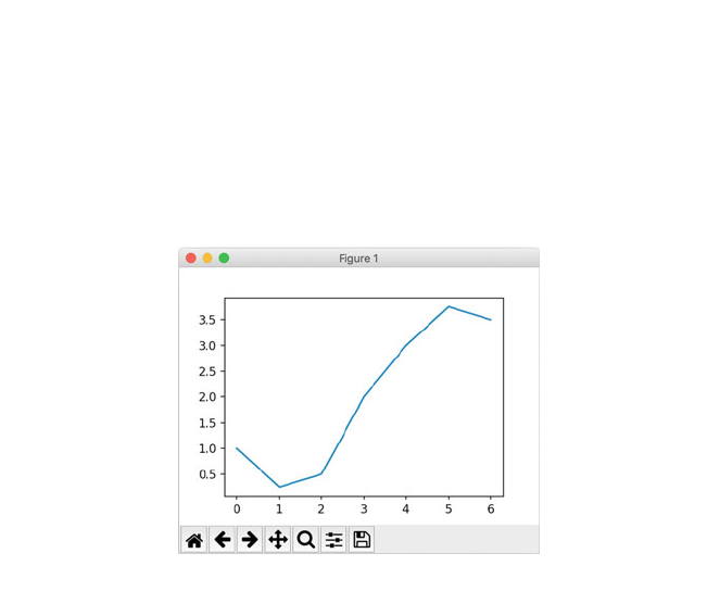
Matplotlib can be used on its own or in conjunction with other libraries to

provide a wide variety of facilities. One library that is often used in conjunction

with Matplotlib is NumPy which is a library often used in Data Science applications

that provides a variety of functions and data structures (such as n-dimensional

arrays) that can be very useful when processing data for display within a chart.

However, Matplotlib does not come prebuilt into the Python environment; it is

an optional module which must be added to your environment or IDE.

In this chapter we will introduce the Matplotlib library, its architecture, the

components that comprise a chart and the pyplot API. The pyplot API is the

simplest and most common way in which a programmer interacts with Matplotlib.

We will then explore a variety of different types of chart and how they can be

created using Matplotlib, from simple line charts, through scatter charts, to bar

charts and pie charts. We will ﬁnish by looking at a simple 3D chart.

5.2 Matplotlib

Matplotlib is a graph plotting library for Python. For simple graphs Matplotlib is

very easy to use, for example to create a simple line graph for a set of x and y

coordinates you can use the matplotlib.p yplot.plot function:

This very simple program generates the following graph:

pyplot.plot([1, 0.25, 0.5, 2, 3, 3.75, 3.5])

# Display the chart in a window

pyplot.show()

import matplotlib.pyplot as pyplot

# Plot a sequence of values

36 5 Introduction to Matplotlib

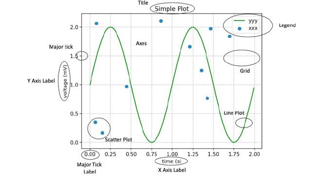
In this example, the plot() function takes a sequence of values which will be

treated as the y axis values; the x axis values are implied by the position of the y

values within the list. Thus as the list has six elements in it the x axis has the range

0–6. In turn as the maximum value contained in the list is 3.75, then the y axis

ranges from 0 to 4.

5.3 Plot Components

Although they may seem simple, there are numerous elements that comprise a

Matplotlib graph or plot. These elements can all be manipulated and modiﬁed

independently. It is therefore useful to be familiar with the Matplotlib terminology

associated with these elements, such as ticks, legends, labels etc.

The elements that make up a plot are illustrated below:

The diagram illustrates the following elements:

• Axes An Axes is deﬁned by the matplotlib.axes.Axes class. It is used to

maintain most of the elements of a ﬁgure namely the X and Y Axis, the Ticks,

the Line plots, any text and any polygon shapes.

• Title This is the title of the whole ﬁgure.

• Ticks (Major and Minor) The Ticks are represented by the class mat-

plotlib.axis .Tick. A Tick is the mark on the Axis indicating a new

5.2 Matplotlib 37

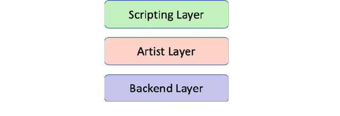
value. There can be Major ticks which are larger and may be label ed. There are

also minor ticks which can be smaller (and may also be labelled).

• Tick Labels (Major and Minor) This is a label on a Tick.

• Axis The maplotlib.axis.Axis class deﬁnes an Axis object (such as an X

or Y axis) within a parent Axes instance. It can have formatters used to format

the labels used for the major and minor ticks. It is also possible to set the

locations of the major and minor ticks.

• Axis Labels (X, Y and in some cases Z) These are labels used to describe the

Axis.

• Plot types such as line and scatter plots. Various types of plots and graphs are

supported by Matplotlib including line plots, scatter graphs , bar charts and pie

charts.

• Grid This is an optional grid displayed behind a plot, graph or chart. The grid

can be displayed with a variety of different line styles (such as solid or dashed

lines), colours and line widths.

5.4 Matplotlib Architecture

The Matplotlib library has a layered architecture that hides much of the complexity

associated with different windowing systems and graphic outputs. This architecture

has three main layers, the Scripting Layer, the Artist Layer and the Backend Layer.

Each layer has speciﬁc responsibilities and components. For example, the Bac kend

is responsible for reading and interacting with the graph or plot being generated. In

turn the Artist Layer is responsible for creating the graph objects that will be

rendered by the Backend Layer. Finally the Scripting Layer is used by the devel-

oper to create the graphs.

This architecture is illustrated below:

38 5 Introduction to Matplotlib

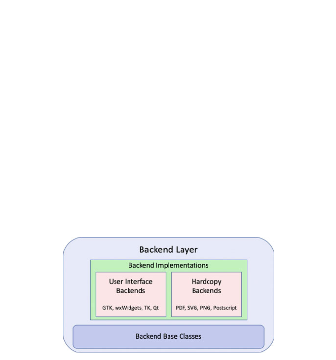
5.4.1 Backend Layer

The Matplotlib backend layer handles the generation of output to different target

formats. Matplotlib itself can be used in many different ways to generate many

different outputs.

Matplotlib can be used interactively, it can be embedded in an application (or

graphical user interface), it may be used as part of a batch application with plots

being stored as PNG, SVG, PDF or other images etc.

To support all of these use cases, Matplotlib can target different outputs, and

each of these capabilities is called a backend; the “frontend” is the developer facing

code. The Backend Layer maintains all the different backends and the programmer

can either use the default backend or select a different backend as required.

The backend to be used can be set via the matplotlib.use() function. For

example, to set the backend to render Postscript use: matplotlib.use(‘PS’) this is

illustrated below:

It should be noted that if you use the matplotlib.use() function, this must

be done before importing matplotlib.pyplot. Calling matplotlib.use

() after matplotlib.pyplot has been imported will have no effect. Note that

the argument passed to the matplotlib.use() function is case sensitive.

The default renderer is the ‘Agg’ which uses the Anti-Grain Geometry C++

library to make a raster (pixel) image of the ﬁgure. This produces high quality raster

graphics based images of the data plots.

The ‘Agg’ backend was chosen as the default backend as it works on a broad

selection of Linux systems as its supporting requirements are quite small; other

backends may run on one particular system, but may not work on another system.

This occurs if a particular system does not have all the dependencies loaded that the

speciﬁed Matplotlib backend relies on.

import matplotlib

if 'matplotlib.backends' not in sys.modules:

matplotlib.use('PS')

import matplotlib.pyplot as pyplot

5.4 Matplotlib Architecture 39

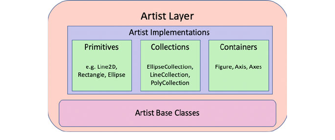
The Backend Layer can be divided into two categories:

• User interface backends (interactive) that support various Python windowing

systems such as wxWidgets (discussed in the next chapter), Qt, TK etc.

• Hardcopy Backends (non interactive) that support raster and vector graphic

outputs.

The User Interface and Hardcopy backends are built upon common abstractions

referred to as the Backend base classes.

5.4.2 The Artist Layer

The Artist layer provides the majority of the functionality that you might consider

to be what Matplotlib actually does; that is the generation of the plots and graphs

that are rendered/ displayed to the user (or output in a particular format).

The artist layer is concerned with things such as the lines, shapes, axis, and axes,

text etc. that comprise a plot.

The classes used by the Artist Layer can be classiﬁed into one of the following

three groups; primitives, containers and collections:

• Primitives are classes used to represent graphical objects that will be drawn on

to a ﬁgures canvas.

• Containers are objects that hold primitives. For example, typically a ﬁgure

would be instantiated and used to create one or more Axes etc.

• Collections are used to efﬁciently handle large numbers of similar types of

objects.

Although it is useful to be aware of these classes; in many cases you will not

need to work with them directly as the pyplot API hides much of the detail.

However, it is possible to work at the level of ﬁgures, axes, ticks etc. if required.

40 5 Introduction to Matplotlib

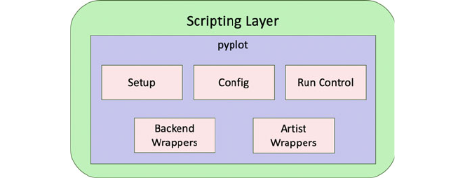
5.4.3 The Scripting Layer

The scripting layer is the developer facing interface that simpliﬁes the task of

working with the other layers.

Note that from the programmers point of view, the Scripting Layer is represented

by the pyplot module. Under the covers pyplot uses module-level objects to

track the state of the data, handle drawing the graphs etc.

When imported pyplot selects either the default backend for the system or the

one that has been conﬁgured; for example via the matplotlib.use() function.

It then calls a setup() function that:

• creates a ﬁgure manager factory function, which when called will create a new

ﬁgure manager appropriate for the selected backend,

• prepares the drawing function that should be used with the selected backend,

• identiﬁes the callable function that integrates with the backend mainloop

function,

• provides the module for the selected backend.

The pyplot interface simpliﬁes interactions with the internal wrappers by

providing methods such as plot(), pie(), bar(), title(), saveﬁg(),

draw() and ﬁgure() etc.

Most of the examples presented in the next chapter will use the functions pro-

vided by the pyplot module to create the required charts; thereby hiding the lower

level details.

5.4 Matplotlib Architecture 41

5.5 Online Resources

See the online documentation for:

•

https://matplotlib.org The Matplotlib library. This incorporates numerous

examples with complete listings, documentation, galleries and a detailed user

guide and FAQ.

•

https://pythonprogramming.net/matplotlib-python-3-basics-tutorial Python Mat-

plotlib crash course.

42 5 Introduction to Matplotlib

Chapter 6

Graphing with Matplotlib pyplot

6.1 Introduction

In this chapter we will explore the Matplotlib pyplot API. This is the most common

way in which developers generate different types of graphs or plots using

Matplotlib.

6.2 The pyplot API

The purpose of the pyplot module and the API it presents is to simplify the

generation and manipulation of Matplotlib plots and charts. As a whole the

Matplotlib library tries to make simple things easy and complex things possible. The

primary way in which it achieves the ﬁrst of these aims is through the py plot API

as this API has high level functions such as bar(), plot(), scatter() and

pie() that make it easy to create bar charts, line plots, scatter graphs and pie charts.

One point to note about the functions provided by the pyplot API is that they

can often take very many parameters; however most of these parameters will have

default values that in many situations will give you a reasonable default behaviour/

default visual repres entation. You can therefore ignore most of the parameters

available until such time as you actually need to do something different; at which

point you should refer to the Matplotlib documentation as this has extensive

material as well as numerous examples.

It is of course necessary to import the pyplot module; as it is a module within

the Matplotlib (e.g. matplotlib.pyplot) library. It is often given an alias

within a program to make it easier to reference. Common alias for this module are

pyplot or plt.

A typical import for the pyplot module is given below:

import matplotlib.pyplot as pyplot

J. Hunt, Advanced Guide to Python 3 Programming,

Undergraduate Topics in Computer Science,

https://doi.org/10.1007/978-3-030-25943-3_6

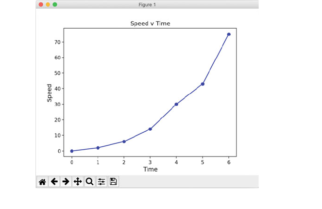
The plyplot API can be used to

• construct the plot,

• conﬁgure labels and axis,

• manage color and line styles,

• handles events/allows plots to be interactive,

• display (show) the plot.

We will see examples of using the pyplot API in the following sections.

6.3 Line Graphs

A Line Graph or Line Plot is a graph with the points on the graph (often referred to

as markers) connected by lines to show how something changes in value as some

set of values (typically the x axis) changes; for example, over a series to time

intervals (also known as a time series). Time Series line charts are typically drawn

in chronological order; such charts are known as run charts.

The following chart is an example of a run chart; it charts time across the bottom

(x axis) against speed (represented by the y axis).

44 6 Graphing with Matplotlib pyplot

The program used to generate this chart is given below:

import matplotlib.pyplot as pyplot

Set up the data

x = [0, 1, 2, 3, 4, 5, 6]

y = [0, 2, 6, 14, 30, 43, 75]

# Set the axes headings

pyplot.ylabel('Speed', fontsize=12)

pyplot.xlabel('Time', fontsize=12)

# Set the title

pyplot.title("Speed v Time")

# Plot and display the graph

# Using blue circles for markers ('bo')

# and a solid line ('-')

pyplot.plot(x, y, 'bo-')

pyplot.show()

The ﬁrst thing that this program does is to import the matplotlib.pyplot

module and give it an alias of pyplot (as this is a shorter name it makes the code

easier to read).

Two lists of values are then created for the x and y coordinates of each marker or

plot point.

The graph itself is then conﬁgured wi th labels being provided for the x and y

axis (using the pyplot functions xlabel() and ylabel()). The title of the graph

is then set (again using a pyplot function).

After this the x and y values are then plotted as a line chart on the graph. This is

done using the pyplot.plot() function. This function can take a wide range of

parameters, the only compulsory parameters being the data used to deﬁne the plot

points. In the above example a third parameter is provided; this is a string ‘bo-’.

This is a coded format string in that each element of the string is meaningful to the

pyplot.plot() function. The elements of the string are:

• b—this indicates the colour to use when drawing the line; in this case the letter

‘b’ indicates the colour blue (in the same way ‘r’ would indicate red and ‘ g ’

would indicate green).

• o—this indicates that each marker (each point being plotted) should be repre-

sented by a cirlce. The lines between the markers then create the line plot.

• ‘–’—This indicates the line style to use. A single dash (‘-’) indicates a solid line,

where as a double dash (‘–’) indicates a dashed line.

6.3 Line Graphs 45

Finally the program then uses the show() function to render the ﬁgure on the

screen; alternatively saveﬁg() could have been used to save the ﬁgure to a ﬁle.

6.3.1 Coded Format Strings

There are numerous options that can be provided via the format string, the fol-

lowing tables summarises some of these:

The following colour abbreviations are supported by the format string:

Character Color

‘b’ blue

‘g’ green

‘r’ red

‘c’ cyan

‘m’ magenta

‘y’ yellow

‘k’ black

‘w’ white

Different ways of representing the markers (points on the graph) connected by

the lines are also supported including:

Character Description

‘.’ point marker

‘,’ pixel marker

‘o’ circle marker

‘v’ triangle_down marker

‘^’ triangle_up marker

‘ < ’ triangle_left marker

‘ > ’ triangle_right marker

‘s’ square marker

‘p’ pentagon marker

‘*’ star marker

‘h’ hexagon1 marker

‘ + ’ plus marker

‘x’ x marker

‘D’ diamond marker

46 6 Graphing with Matplotlib pyplot

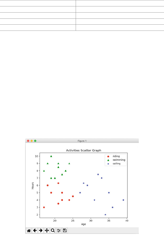
Finally, the format string supports different line styles:

Character Description

‘-’ solid line style

‘–’ dashed line style

‘-.’ dash-dot line style

‘:’ dotted line style

Some examples of formatting strings:

• ‘r’ red line with default markers and line style.

• ‘g-’ green solid line.

• ‘–’ dashed line with the default colour and default markers.

• ‘yo:’ yellow dotted line with circle markers.

6.4 Scatter Graph

A Scatter Graph or Scatter Plot is type of plot where individual values are indicated

using cartesian (or x and y) coordinates to display values. Each value is indicated

via a mark (such as a circle or triangle) on the graph. They can be used to represent

values obtained for two different variables; one plotted on the x axis and the other

plotted on the y axis.

An example of a scatter chart with three sets of scatter values is given below

6.3 Line Graphs 47

In this graph each dot represents the amount of time people of different ages

spend on three different activities.

The program that was used to generate the above graph is shown below:

In the above example the plot.scatter() function is used to generate the

scatter graph for the data deﬁned by the riding, swimming and sailing tuples.

The colours of the markers have been speciﬁed using the named parameter c.

This parameter can take a string representing the name of a colour or a two

dimensional array with a single row in which each value in the row represents an

RGB color code. The marker Indicates the marker style such as ‘o ’ for a circle, a

‘^’ for a triangle and ‘*’ for a star shape. The label is used in the chart legend for

the marker.

Other options available on the pyplot.sca tter() function include:

• alpha : indicates the alpha blending value, between 0 (transparent) and 1

(opaque).

import matplotlib.pyplot as pyplot

# Create data

riding = ((17, 18, 21, 22, 19, 21, 25, 22, 25, 24),

(3, 6, 3.5, 4, 5, 6.3, 4.5, 5, 4.5, 4))

swimming = ((17, 18, 20, 19, 22, 21, 23, 19, 21, 24),

(8, 9, 7, 10, 7.5, 9, 8, 7, 8.5, 9))

sailing = ((31, 28, 29, 36, 27, 32, 34, 35, 33, 39),

(4, 6.3, 6, 3, 5, 7.5, 2, 5, 7, 4))

# Plot the data

pyplot.scatter(x=riding[0], y=riding[1], c='red', marker='o',

label='riding')

pyplot.scatter(x=swimming[0], y=swimming[1], c='green',

marker='^', label='swimming')

pyplot.scatter(x=sailing[0], y=sailing[1], c='blue',

marker='*', label='sailing')

# Configure graph

pyplot.xlabel('Age')

pyplot.ylabel('Hours')

pyplot.title('Activities Scatter Graph')

pyplot.legend()

pyplot.show()

# Display the chart

48 6 Graphing with Matplotlib pyplot

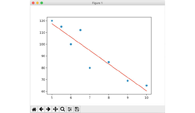
• linewidths : which is used to indicate the line width of the marker edges.

• edgecolors : indicates the color to use for the marker edges if different from

the ﬁll colour used for the marker (indicates by the parameter ‘c’).

6.4.1 When to Use Scatter Graphs

A useful question to consider is when should a scatter plot be used? In general

scatter plats are used when it is necessary to show the relationship between two

variables. Scatter plots are sometimes called correlation plots because they show

how two variables are correlated.

In many cases a trend can be discerned between the points plotted on a scatter

chart (although there may be outlying values). To help visualise the trend it can be

useful to draw a trend line along with the scatter graph. The trend line helps to make

the relationship of the scatter plots to the general trend clearer.

The following chart represents a set of values as a scatter graph and draws the

trend line of this scatter graph. As can be seen some values are closer to the

trendline than others.

The trend line has been created in this case using the numpy function polyﬁt().

6.4 Scatter Graph 49

The polyﬁt() function performs a least squares polynomial ﬁt for the data it is

given. A poly1d class is then created based on the array returned by polyﬁt().

This class is a one-dimensional polynomial class. It is a convenience class , used to

encapsulate “natural” operations on polynomials. The poly1d object is then used

to generat e a set of values for use with the set of x values for the function py-

plot.plot().

import numpy as np

import matplotlib.pyplot as pyplot

x = (5, 5.5, 6, 6.5, 7, 8, 9, 10)

y = (120, 115, 100, 112, 80, 85, 69, 65)

# Generate the scatter plot

pyplot.scatter(x, y)

# Generate the trend line

z = np.polyfit(x, y, 1)

p = np.poly1d(z)

pyplot.plot(x, p(x), 'r')

# Display the figure

pyplot.show()

6.5 Pie Charts

A Pie Chart is a type of graph in which a circle is divided into sectors (or wedges)

that each represent a proportion of the whole. A wedge of the circle represents a

category’s contribution to the overall total. As such the graph resembles a pie that

has been cut into different sized slices.

Typically, the different sectors of the pie chart are presented in different colours

and are arranged clockwise around the chart in order of magnitude. However, if

there is a slice that does not contain a unique category of data but summarises

several, for example “other types” or “other answers”, then even if it is not the

smallest category, it is usual to display it last in order that it does not detract from

the named categories of interest.

50 6 Graphing with Matplotlib pyplot

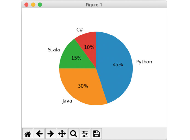
The following chart illustrates a pie chart used to represent programming lan-

guage usage within a particular organisation.

The pie chart is created using the pyplot.pie() function.

import matplotlib.pyplot as pyplot

labels = ('Python', 'Java', 'Scala', 'C#')

sizes = [45, 30, 15, 10]

pyplot.pie(sizes,

labels=labels,

autopct='%1.f%%',

counterclock=False,

startangle=90)

pyplot.show()

The pyplot.pie() function takes several parameters, most of which are

optional. The only required parameter is the ﬁrst one that provides the values to be

used for the wedge or segment sizes. The following optional parameters are used in

the above example:

6.5 Pie Charts 51

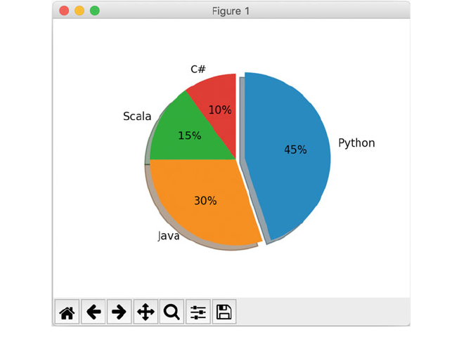
• The labels parameter is an optional parameter that can take a sequence of

strings that are used to provide labels for each wedge.

• The autopct parameter takes a string (or function) to be used to format the

numeric values used with each wedge.

• The counterclockwise parameter. By default wedges are plotted counter

clockwise in pyplot and so to ensure that the layout is more like the traditional

clockwise approach the counterc lock parameter is set to False.

• The startangle parameter. The starting angle has also been moved 90°

using the startangle parameter so that the ﬁrst segment starts at the top of

the chart.

6.5.1 Expanding Segments

It can be useful to emphasis a particular segment of the pie chart by exploding it;

that is separating it out from the rest of the pie chart. This can be d one using the

explode parameter of the pie() function that takes a sequence of values indi-

cating how much a segment should be exploded by.

The visual impact of the pie chart can also be enhanced in this case by adding a

shadow to the segments using the named shadow boolean parameter. The effect of

these are shown below:

52 6 Graphing with Matplotlib pyplot

The program that generated this modiﬁed chart is given below for reference:

import matplotlib.pyplot as pyplot

labels = ('Python', 'Java', 'Scala', 'C#')

sizes = [45, 30, 15, 10]

# only "explode" the 1st slice (i.e. 'Python')

explode = (0.1, 0, 0, 0)

pyplot.pie(sizes,

explode=explode,

labels=labels,

autopct='%1.f%%',

shadow=True,

counterclock=False,

startangle=90)

pyplot.show()

6.5.2 When to Use Pie Charts

It is useful to consider what data can be/should be presented using a pie chart. In

general pie charts are useful for displaying data that can be classiﬁed into nominal

or ordinal categories. Nominal data is categorised according to descriptive or

qualitative information such as program languages, type of car, country of birth etc.

Ordinal data is similar but the categories can also be ranked, for example in a

survey people may be asked to say whether they classed something as very poor,

poor, fair, good, very good.

Pie charts can also be used to show percentage or proportional data and usually

the percentage represented by each category is provided next to the corresponding

slice of pie.

Pie charts are also typically limited to presenting data for six or less categories.

When there are more categories it is difﬁcult for the eye to distinguish between the

relative sizes of the different sectors and so the chart becomes difﬁcult to interpret.

6.5 Pie Charts 53

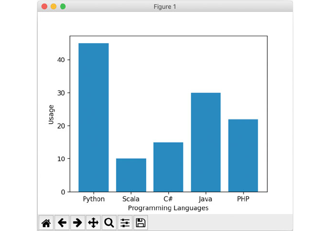
6.6 Bar Charts

A Bar Chart is a type of chart or graph that is used to present different discrete

categories of data. The data is usually presented vertically although in some cases

horizontal bar charts may be used. Each category is represented by a bar whose

height (or length) represents the data for that category.

Because it is easy to interpret bar charts, and how each category relates to another,

they are one of the most commonly used types of chart. There are also several

different common variations such as grouped bar charts and stacked bar charts.

The following is an example of a typical bar chart. Five categories of pro-

gramming languages are presented along the x axis while the y axis indicates

percentage usage. Each bar then represents the usage percentage associated with

each programming language.

The program used to generate the above ﬁgure is given below:

54 6 Graphing with Matplotlib pyplot

# Set up the data

labels = ('Python', 'Scala', 'C#', 'Java', 'PHP')

index = (1, 2, 3, 4, 5) # provides locations on x axis

sizes = [45, 10, 15, 30, 22]

# Set up the bar chart

pyplot.bar(index, sizes, tick_label=labels)

# Configure the layout

pyplot.ylabel('Usage')

pyplot.xlabel('Programming Languages')

# Display the chart

pyplot.show()

import matplotlib.pyplot as pyplot

The chart is constructed such that the lengths of the different bars are propor-

tional to the size of the category they represent. The x-axis represents the different

categories and so has no scale. In order to emphasise the fact that the categories are

discrete, a gap is left between the bars on the x-axis. The y-axis does have a scale

and this indicates the units of measurement.

6.6.1 Horizontal Bar Charts

Bar charts are normally drawn so that the bars are vertical which means that the

taller the bar, the larger the category. However , it is also possible to draw bar charts

so that the bars are horizontal which means that the longer the bar, the larger the

category. This is a particularly effective way of presenting a large number of

different categories when there is insufﬁcient space to ﬁt all the columns required

for a vertical bar chart across the page.

In Matplotlib the pyplot.barh() function can be used to generate a hori-

zontal bar chart:

6.6 Bar Charts 55

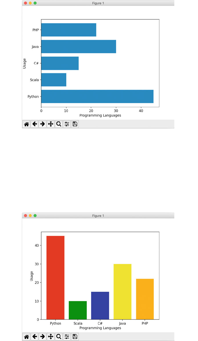
In this case the only line of code to change from the previous example is:

pyplot.barh(x_values, sizes, tick_label = labels)

6.6.2 Coloured Bars

It is also common to colour different bars in the chart in different colours or using

different shades. This can help to distinguish one bar from another. An example is

given below:

56 6 Graphing with Matplotlib pyplot

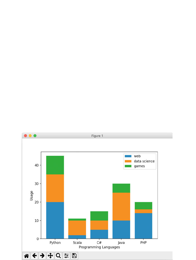
The colour to be used for e ach category can be provided via the color

parameter to the bar() (and barh()) function. This is a sequence of the colours

to apply. For example, the above coloured bar chart can be generated using:

6.6.3 Stacked Bar Charts

Bar Charts can also be stacked. This can be a way of showing total values (and what

contributes to those total values) across several categories. That is, it is a way of

viewing overall totals, for several different categories based on how different ele-

ments contribute to those totals.

Different colours are used for the different sub-groups that contribute to the

overall bar. In such cases, a legend or key is usually provided to indicate what

sub-group each of the shadings/colours represent. The legend can be placed in the

plot area or may be located below the chart.

For example, in the following chart the total usage of a particular programming

language is composed of its use in games and web development as well as data

science analytics.

From this ﬁgure we can see how much each use of a programming language

contributes to the overall usage of that language. The program that generated this

chart is given below:

pyplot.bar(x_values, sizes, tick_label=labels, color=('red',

'green', 'blue', 'yellow', 'orange'))

6.6 Bar Charts 57

One thing to note from this example is that after the ﬁrst set of values are added

using the pyplot.bar() function, it is necessary to specify the bottom locations

for the next set of bars using the bottom parameter. We can do this just using the

values already used for web_usage for the second bar chart; however for the third

bar chart we must add the values used for web_usage and data_-

science_usage together (in this case using a for list comprehension).

6.6.4 Grouped Bar Charts

Finally, Grouped Bar Charts are a way of showing information about different

sub-groups of the main categories. In such cases, a legend or key is usually pro-

vided to indicate what sub-group each of the shadings/colours represent. The legend

can be placed in the plot area or may be located below the chart.

For a particular category separate bar charts are drawn for each of the subgro ups.

For example, in the following chart the results obtained for two sets of teams across

import matplotlib.pyplot as pyplot

# Set up the data

labels = ('Python', 'Scala', 'C#', 'Java', 'PHP')

index = (1, 2, 3, 4, 5)

web_usage = [20, 2, 5, 10, 14]

data_science_usage = [15, 8, 5, 15, 2]

games_usage = [10, 1, 5, 5, 4]

# Set up the bar chart

pyplot.bar(index, web_usage, tick_label=labels, label='web')

pyplot.bar(index, data_science_usage, tick_label=labels,

label='data science', bottom=web_usage)

web_and_games_usage = [web_usage[i] + data_science_usage[i]

for

i in range(0, len(web_usage))]

pyplot.bar(index, games_usage, tick_label=labels,

label='games', bottom=web_and_games_usage)

# Configure the layout

pyplot.ylabel('Usage')

pyplot.xlabel('Programming Languages')

pyplot.legend()

# Display the chart

pyplot.show()

58 6 Graphing with Matplotlib pyplot

a series of lab exercises are displayed. Thus each team has a bar for lab1, lab2, lab3

etc. A space is left between each category to make it easier to compare the sub

categories.

The following program generates the grouped bar chart for the lab exercises

example:

Notice in the above program that it has been necessary to calculate the index for

the second team as we want the bars presented next to each other. Thus the index

for the teams includes the width of the bar for each index point, thus the ﬁrst bar is

at index position 1.35, the second at index position 2.35 etc. Finally the tick

positions must therefore be between the two bars and thus is calculated by taking

into account the bar widths.

import matplotlib.pyplot as pyplot

BAR_WIDTH = 0.35

# set up grouped bar charts

teama_results = (60, 75, 56, 62, 58)

teamb_results = (55, 68, 80, 73, 55)

# Set up the index for each bar

index_teama = (1, 2, 3, 4, 5)

index_teamb = [i + BAR_WIDTH for i in index_teama]

# Determine the mid point for the ticks

ticks = [i + BAR_WIDTH / 2 for i in index_teama]

tick_labels = ('Lab 1', 'Lab 2', 'Lab 3', 'Lab 4', 'Lab 5')

# Plot the bar charts

pyplot.bar(index_teama, teama_results, BAR_WIDTH, color='b',

label='Team A')

pyplot.bar(index_teamb, teamb_results, BAR_WIDTH, color='g',

label='Team B')

# Set up the graph

pyplot.xlabel('Labs')

pyplot.ylabel('Scores')

pyplot.title('Scores by Lab')

pyplot.xticks(ticks, tick_labels)

pyplot.legend()

# Display the graph

pyplot.show()

6.6 Bar Charts 59

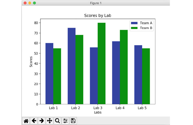
This program generates the following grouped bar chart:

6.7 Figures and Subplots

A Matplotlib ﬁgure is the object that contains all the graphical elements displayed

on a plot. That is the axes, the legend , the title as well as the line plot or bar chart

itself. It thus represents the overall window or page and is the top, out graphical

component.

In many ca ses the ﬁgure is implicit as the developer interacts with the pyplot

API; however the ﬁgure can be accessed directly if required.

The matplotlib.pyplot.ﬁgure() function generates a ﬁgure object.

This function returns a matplotlib.ﬁgure.Figure object. It is then possible

to interact directly with the ﬁgure object. For example it is possible to add axes to

the ﬁgure, to add sub plots to a graph etc.

Working directly with the ﬁgure is necessary if you want to add multiple sub-

plots to a ﬁgure. This can be useful if what is required is to be able to compare

different views of the same data side by side. Each subplot has its own axes which

can coexist within the ﬁgure.

One or more subplots can be added to a ﬁgure using the ﬁgure.add_

subplot() method. This method adds an Axes to the ﬁgure as one of a set of one

or more subplots. A subplot can be added using a 3-digit integer (or three separate

integers) describing the position of the subplot. The digits represent the number of

rows, columns and the index of the sub plot within the resulting matrix.

60 6 Graphing with Matplotlib pyplot

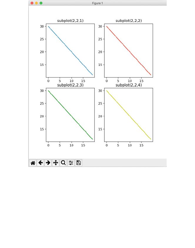
Thus 2, 2, 1 (and 221) all indicate that the subplot will take the 1st index within a

two by two grid of plots. In turn 2, 2, 3 (223) indicates that the sub plot will be at

index 3 which will be row 2 and column 1 within the 2 by 2 grid of plots. Where as

2, 2, 4 (or 224) indicates that the plot should be added as at index 4 or the fourth

subplot within the grid (so position 2 by 2) etc.

For example, the following ﬁgure illustrates four subplots presented within a

single ﬁgure. Each subplot is added via the ﬁgure.add_subplot() method.

6.7 Figures and Subplots 61

This ﬁgure is generated by the following program:

import matplotlib.pyplot as pyplot

t = range(0, 20)

s = range(30, 10, -1)

# Set up the grid of subplots to be 2 by 2

grid_size='22'

# Initialize a Figure

figure = pyplot.figure()

# Add first subplot

position = grid_size + '1'

print('Adding first subplot to position', position)

axis1 = figure.add_subplot(position)

axis1.set(title='subplot(2,2,1)')

axis1.plot(t, s)

# Add second subplot

position = grid_size + '2'

print('Adding second subplot to position', position)

axis2 = figure.add_subplot(position)

axis2.set(title='subplot(2,2,2)')

axis2.plot(t, s, 'r-')

# Add third subplot

position = grid_size + '3'

print('Adding third subplot to position', position)

axis3 = figure.add_subplot(position)

axis3.set(title='subplot(2,2,3)')

axis3.plot(t, s, 'g-')

# Add fourth subplot

position = grid_size + '4'

print('Adding fourth subplot to position', position)

axis4 = figure.add_subplot(position)

axis4.set(title='subplot(2,2,4)')

axis4.plot(t, s, 'y-')

# Display the chart

pyplot.show()

62 6 Graphing with Matplotlib pyplot

The console output from this program is given below:

Adding first subplot to position 221

Adding second subplot to position 222

Adding third subplot to position 223

Adding fourth subplot to position 224

6.8 3D Graphs

A three dimensional graph is used to plot the relationships between three sets of

values (instead of the two used in the examples presented so far in this chapter). In a

three dimensional graph as well as the x and y axis there is also a z axis.

The following program creates a simple 3D graph using two sets o f values

generated using the numpy range function. These are then converted into a

coordinate matrices using the numpy meshgrid() function. The z axis values are

created using the numpy sin() function. The 3D graph surface is plotted using the

plot_surface() function of the futures axes object. This takes the x, y and z

coordinates. The function is also given a colour map to use when rendering the

surface (in this case the Matplotlib cool to warm colour map is used).

# Make the data to be displayed

x_values = np.arange(-6, 6, 0.3)

y_values = np.arange(-6, 6, 0.3)

# Generate coordinate matrices from coordinate vectors

x_values, y_values = np.meshgrid(x_values, y_values)

# Generate Z values as sin of x plus y values

z_values = np.sin(x_values + y_values)

import matplotlib.pyplot as pyplot

# Import matplotlib colour map

from matplotlib import cm as colourmap

# Required for £D Projections

from mpl_toolkits.mplot3d import Axes3D

# Provide access to numpy functions

import numpy as np

6.7 Figures and Subplots 63

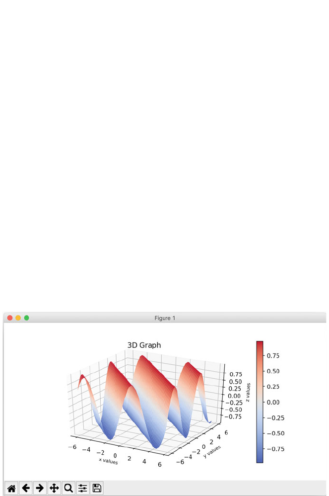
This program generates the following 3D graph:

# Obtain the figure object

figure = pyplot.figure()

# Get the axes object for the 3D graph

axes = figure.gca(projection='3d')

# Plot the surface.

surf = axes.plot_surface(x_values,

y_values,

z_values,

cmap=colourmap.coolwarm)

# Add a color bar which maps values to colors.

figure.colorbar(surf)

# Add labels to the graph

pyplot.title("3D Graph")

axes.set_ylabel('y values', fontsize=8)

axes.set_xlabel('x values', fontsize=8)

axes.set_zlabel('z values', fontsize=8)

# Display the graph

pyplot.show()

64 6 Graphing with Matplotlib pyplot

One point to note about three dimensional graphs is that they are not universally

accepted as being a good way to present data. One of the maxims of data visual-

isation is keep it simple/ keep it clean. Many consider that a three dimensional chart

does not do this and that it can be difﬁcult to see what is really being shown or that

it can be hard to interpret the data appropriately. For example, in the above chart

what are the values associated wi th any of the peaks? This is difﬁcult to determine

as it is hard to see where the peaks are relative to the X, Y and Z axis. Many

consider such 3D charts to be eye candy; pretty to look at but not providing much

information. As such the use of a 3D chart should be minimised and only used

when actually necessary.

6.9 Exercises

The following table provides information on cities in the UK and their populations

(note that London has been omitted as its population is so much larger than that of

any other city and this would distort the graph).

City Population

Bristol 617,280

Cardiff 447,287

Bath 94,782

Liverpool 864,122

Glasgow 591,620

Edinburgh 464,990

Leeds 455,123

Reading 318,014

Swansea 300,352

Manchester 395,515

Using this data create:

1. A scatter plot for the city to population data.

2. A bar chart for the city to population data.

6.8 3D Graphs 65

Chapter 7

Graphical User Interfaces

7.1 Introduction

A Graphical User Interface can capture the essence of an idea or a situation, often

avoiding the need for a long passage of text. Such interfaces can save a user from

the need to learn complex commands. They are less likely to intimidate computer

users and can provide a large amount of information quickly in a form which can be

easily assimilated by the user.

The widespr ead use of high quality graphical interfaces has led many computer

users to expect such interfaces to any software they use. Most programming lan-

guages either incorporate a Graphical User Interface (GUI) library or have third

party libraries available.

Python is of course a cross platform programming language and this brings in

additional complexities as the underlying operating system may provide different

windowing facilities depending upon whether the program is running on Unix,

Linux, Mac OS or Windows operating systems.

In this chapter we will ﬁrst introduce what we mean by a GUI and by WIMP

based UIs in particular. We will then consider the range of libraries available for

Python before selecting one to use. This chapter will then describe how to create

rich client graphical displays (desktop application) using one of these GUI libraries.

Thus in this chapter we consider how windows, buttons, text ﬁelds and labels etc.

are created, added to windows, positioned and organised.

J. Hunt, Advanced Guide to Python 3 Programming,

Undergraduate Topics in Computer Science,

https://doi.org/10.1007/978-3-030-25943-3_7

7.2 GUIs and WIMPS

GUIs (Graphical User Interfaces) and WIMP (Windows, Icons, Mice and Pop-up

Menus) style interfaces have been available within computer systems for many

years but they are still one of the most signiﬁcant developments to have occurred.

These interfaces were originally developed out of a desire to address many of the

perceived weaknesses of purely textual interfaces.

The textual interface to an operating system was typiﬁed by a peremptory

prompt. In Unix/Linux systems for example, the prompt is often merely a single

character such as %, > or $, which can be intimidating. This is true even for

experienced computer users if they are not familiar with the Unix/Linux family of

operating systems.

For example, a user wishing to copy a ﬁle from one directory to another might

have to type something like:

> cp file.pdf ~otheruser/projdir/srcdir/newfile.pdf

This long sequence needs to be entered with no mistakes in order to be accept ed.

Any error in this command will cause the system to generate an error message

which might or might not be enli ghtening. Even where systems attempt to be more

“user friendly’’ through features like command histories, much typing of arrow

keys and ﬁlenames is typically needed.

The main issue on both input and output is one of bandwidth. For example,

in situations where the relationships between large amounts of information must be

described, it is much easier to assimilate this if output is displayed graphically than

if it is displayed as a tables of ﬁgures. On input, combinations of mouse actions can

be given a meaning that could otherwise only be conveyed by several lines of text.

WIMP stands for Windows (or Window Managers), Icons, Mice and Pop-up

menus. WIMP inte rfaces allow the user to overcome at least some of the weak-

nesses of their textual counterparts—it is possible to provide a pictorial image of the

operating system which can be based on a concept the user can relate to, menus can

be used instead of textual commands and information in general can be displayed

graphically.

The fundamental concepts presented via a WIMP interface were originally

developed at XEROX’s Palo Alto Research Center and used on the Xerox Star

machine, but gained much wider acceptance through ﬁrst the Apple Macintosh and

then IBM PC implementations of WIMP interfaces .

Most WIMP style environmen ts use a desktop analogy (although this is less true

of mobile devices such as phones and tablets):

• the whole screen represents a working surface (a desktop),

• graphic windows that can overlap represent sheets of paper on that desktop,

68 7 Graphical User Interfaces

• graphic objects are used for speciﬁc concepts, for example ﬁling cabinets for

disks or a waste bin for ﬁle disposal (these could be regarded as desk

accessories),

• various application programs are displayed on the screen, these stand for tools

that you might use on your desktop.

In order to interact with this display, the WIMP user is provided with a mouse

(or a light pen or a touch sensitive screen), which can be used to select icons and

menus or to manipulate windows.

The software basis of any WIMP style environment is the window manager. It

controls the multiple, possibly overlapping windows and icons displayed on the

screen. It also handles the transfer of information about events which occur in those

windows to the appropriate application and generates the various menus and

prompts used.

A window is an area of the graphic screen in which a page or piece of a page of

information may be displayed; it may display text, graphics or a combination of

both. These windows may be overlapping, and associated with the same process, or

they may be associated with separate processes. Windows can generally be created,

opened, closed, moved and resized.

An icon is a small graphic object that is usually symbolic of an operation or of a

larger entity such as an application program or a ﬁle. The opening of an icon causes

either the associated application to execute or the associated window to be

displayed.

At the heart of the users ability to interact with such WIMP based programs is

the event loop. This loop listens for events such as the user clicking a button or

selecting a menu item or entering a text ﬁeld. When such an event occurs it triggers

the associated behaviour (such as running a function linked with a button).

7.3 Windowing Frameworks for Python

Python is a cross platform programming language. As such Python programs can be

written on one platform (such as a Linux box) and then run on that platform or

another operating system platform (such as Windows or Mac OS). This can

however generate issues for libraries that need to be available across multiple

operating system platforms. The area of GUIs is particularly an issue as a library

written to exploit features available in the Microsoft Windows system may not be

available (or may look different) on Mac OS or Linux systems.

Each operat ing system that Python runs on may have one or more windowing

systems written for it and these systems may or may not be available on other

operating systems. This makes the job of providing a GUI library for Python that

much more difﬁcult.

7.2 GUIs and WIMPS 69

Developers of Python GUIs have taken one of two approaches to handle this:

• One approach is to write a wrapper that abstracts the underlying GUI facilities

so that the developer works at a level above a speciﬁc windowing system’s

facilities. The Python library then maps (as best it can) the facilities to the

underlying system that is currently being used.

• The other approach is to provide a closer wrapping to a particular set of facilities

on the underlying GUI system and to only target systems that support those

facilities.

Some of the libraries available for Python are listed below and have been cat-

egorised into platform-independent libraries and platform-speciﬁc libraries:

7.3.1 Platform-Independent GUI Libraries

• Tkinter. This is the standard built-in Python GUI library. It is built on top of the

Tcl/Tk widget set that has been around for very many years for many different

operating systems. Tcl stands for Tool Command Language while Tk is the

graphical user interface toolkit for Tcl.

• wxPython. wxWidgets is a free, highly portable GUI library. Its is written in C+

+ and it can provi de a native look and feel on operating systems such as

Windows, Mac OS, Linux etc. wxPython is a set of Python bindings for

wxWidgets. This is the library that we will be using in this chapter.

• PyQT or PySide both of these libraries wrap the Qt toolkit facilities. Qt is a

cross platform software development system for the implementation of GUIs

and applications.

7.3.2 Platform-Speciﬁc GUI Libraries

• PyObjc is a Mac OS speciﬁc library that provides an Objective-C bridge to the

Apple Mac Cocoa GUI libraries.

• PythonWin provides a set of wrappings around the Microsoft Windows

Foundation classes and can be used to create Windows based GUIs.

70 7 Graphical User Interfaces

7.4 Online Resources

There are numerous online references that support the development of GUIs and of

Python GUIs in particular, including:

•

https://www.wxpython.org wxPython home page.

•

https://www.tcl.tk for Infor mation on Tcl/Tk.

•

https://www.qt.io For information on the Qt cross-platform software and UI

development library.

•

https://wiki.python.org/moin/PyQt For information about PyQt.

•

https://pypi.org/project/PySide/ which provides project information for PySide.

•

https://en.wikipedia.org/wiki/Cocoa_(API ) for the Wikipedia page on the

MacOS Cocoa library.

•

https://pythonhosted.org/pyobjc/ for information on the Python to Objective-C

bridge.

•

https://docs.microsoft.com/en-us/cpp/mfc/mfc-desktop-applications?view=vs-

2019

Provides an introduction to the Microsoft Foundation classes.

•

https://www.cgl.ucsf.edu/Outreach/pc204/pythonwin.html for information on

PythonWin.

7.4 Online Resources 71

Chapter 8

The wxPython GUI Library

8.1 The wxPython Library

The wxPython library is a cross platform GUI library (or toolkit) for Python. It

allows programmers to develop highly graphical user interfaces for their programs

using common concepts such as menu bars, menus, buttons, ﬁelds, panels and

frames.

In wxPython all the elements of a GUI are contained within top level windows

such as a wx.Frame or a wx.Dialog. These window s contain graphical com-

ponents known as widgets or controls. These widgets/controls may be grouped

together into Panels (which may or may not have a visible representation).

Thus in wxPython we might construct a GUI from:

• Frames which provide the basic structure for a window: borders, a label and

some basic functionality (e.g. resizing).

• Dialogs which are like Frames but provide fewer border controls.

• Widgets/Controls that are graphical objects displayed in a frame. Some other

languages refer to them as UI components. Examples of widgets are buttons,

checkboxes, selection lists, labels and text ﬁelds.

• Containers are component that are made up of one or more other components

(or containers). All the components within a container (such as a panel) can be

treated as a single entity.

Thus a GUI is constructed hierarchically from a set of widgets, containers and

one or more Frames (or in the case of a pop up dialog then Dialogs). This is

illustrated below for a window containing several panels and widgets:

J. Hunt, Advanced Guide to Python 3 Programming,

Undergraduate Topics in Computer Science,

https://doi.org/10.1007/978-3-030-25943-3_8

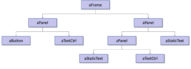
Windows such as Frames and Dialogs have a component hierarchy that is used

(amongst other things) to determine how and when elements of the window are

drawn and redrawn. The component hierarchy is rooted with the frame, within

which components and containers can be added.

The above ﬁgure illustrates a component hierarchy for a frame, with two con-

tainer Panels and a few basic widgets/ui components held within the Panels. Note

that a panel can contain another sub panel with different widgets in.

8.1.1 wxPython Modules

The wxPython library is comprised of many different modules. These modules

provide different features from the core wx module to the html oriented wx.html

and wx.html2 modules. These modules include:

• wx which holds the core widgets and classes in the wx library.

• wx.adv that provides less commonly used or more advanced widgets and

classes.

• wx.grid contains widgets and classes supporting the display and editing of

tabular data.

• wx.richtext consists of widgets and classes used for displaying multiple

text styles and images.

• wx.html comprises widgets and supporting classes for a generic html renderer.

• wx.html2 provides further widget and supporting classe s for a native html

renderer, with CSS and javascript support.

74 8 The wxPython GUI Library

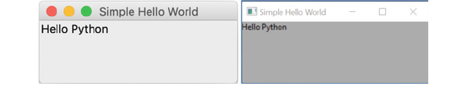
8.1.2 Windows as Objects

In wxPython, Frames and Dialogs as well as their contents are instances of

appropriate classes (such as Frame, Dialog, Panel, Button or

StaticText). Thus when you create a window, you create an object that knows

how to display itself on the computer screen. You must tell it what to display and

then tell it to show its contents to the user.

You should bear the following points in mind during your reading of this

chapter; they will help you understand what you are required to do:

• You create a window by instantiating a Frame or Dialog object.

• You deﬁne what the window displays by creating a widget that has an appro-

priate parent component. This adds the widget to a container, such as a type of

panel or a frame.

• You can send messages to the window to change its state, perform an operation,

and display a graphic object.

• The window, or components within the window, can send messages to other

objects in response to user (or program) actions.

• Everything displayed by a window is an instance of a class and is potentially

subject to all of the above.

• wx.App handles the main event loop of the GUI application.

8.1.3 A Simple Example

An example of creating a very simple window using wxPython is given below. The

result of running this short program is shown here for both a Mac and a Windows

PC:

This program creates a top level window (the wx.Frame) and gives it a title. It

also creates a label (a wx.StaticText object) to be displayed within the frame.

8.1 The wxPython Library 75

To use the wxPython library it is necessary to import the wx module.

The program also creates a new instance of the Application Object called wx.

App().

Every wxPython GUI program must have one Application Object. It is the

equivalent of the main() function in many non-GUI applications as it will run the

GUI application for you. It also provides default facilities for deﬁning startup and

shutdown operations and can be subclassed to create custom behaviour.

The wx.StaticText class is used to create a single (or multiple) line label. In

this case the label shows the string ‘Hello Python’. The StaticText object is

constructed with reference to its parent container. This is the container within which

the text will be displayed. In this case the StaticText is being displayed directly

within the Frame and thus the frame object is its containing parent object. In

contrast the Frame which is a top level window, does not have a parent container.

Also notice that the frame must be shown (displayed) for the user to see it. This

is because there might be multiple different windows that need to be shown (or

hidden) in different situations for an application.

Finally the program starts the applications’ main event loop; within this loop the

program listens for any user input (such as requesting that the window is closed).

8.2 The wx.App Class

The wx.App class represents the application and is used to:

• start up the wxPython system and initialise the underlying GUI toolkit,

• set and get application-wide properties,

• implement the native windowing system main message or event loop, and to

dispatch events to window instances.

import wx

# Create the Application Object

app = wx.App()

# Now create a Frame (representing the window)

frame = wx.Frame(parent=None, title=' Simple Hello World')

# And add a text label to it

text = wx.StaticText(parent=frame, label= 'Hello Python')

# Display the window (frame)

frame.Show()

# Start the event loop

app.MainLoop()

76 8 The wxPython GUI Library

Every wxPython application must have a single wx.App instance. The creation

of all of the UI objects should be delayed until after the wx.App object has been

created in order to ensure that the GUI platform and wxWidgets have been fully

initialised.

It is common to subclass the wx.App class and override methods such as

OnPreInit and OnExi t to provide custom behaviour. This ensures that the

required behaviour is run at appropriate times. The methods that can be overridden

for this purpose are:

• OnPreInit, This met hod can be overridden to deﬁne behaviour that should be

run once the application object is created, but before the OnInit method has been

called.

• OnInit This is expected to create the applications main window , display that

window etc.

• OnRun, This is the method used to start the execution of the main program.

• OnExit, This can be overridden to provide any behaviour that should be called

just before the application exits.

As an example, if we wish to set up a GUI application such that the mai n frame

is initialised and shown after the wx.Ap p has been instantiated then the safest way

is to override the OnInit() method of the wx.App class in a suitable subclass.

The method should return True of False; where True is used to indicate that

processing of the application should continue and False indicates that the

application should terminate immediately (usually as the result of some unexpected

issue).

An example wx.App subclass is shown below:

This class can now be instantiated and the MainLoop started, for example:

It is also possible to override the OnExit() to clean up anything initialised in

the OnInit() method.

class MainApp(wx.App):

def OnInit(self):

""" Initialise the main GUI Application"""

frame = WelcomeFrame()

frame.Show()

# Indicate whether processing should continue or no

return True

# Run the GUI applicatio

app = MainApp()

app.MainLoop()

8.2 The wx.App Class 77

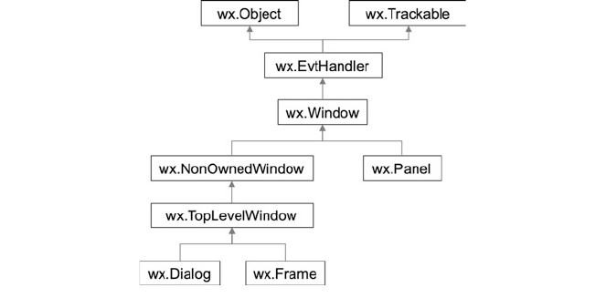
8.3 Window Classes

The window or widget container classes that are commonly used within a

wxPython application are:

• wx.Dialog A Dialog is a top level window used for popups where the user

has limited ability to interact with the window. In many cases the user can only

input some data and/or accept or decline an option.

• wx.Frame A Frame is a top level window whose size and position can be set

and can (usually) be controlled by the user.

• wx.Panel Is a container (non top level window) on which controls/widgets

can be placed. This is often used in conjunction with a Dialog or a Frame to

manage the positioning of widgets within the GUI.

The inheritance hierarchy for these classes is given below for reference:

As an example of using a Frame and a Panel, the following application

creates two Panels and displays them within a top level Frame. The background

colour of the Frame is the default grey; while the background colour for the ﬁrst

Panel is blue and for the second Panel it is red. The resulting display is shown

below:

78 8 The wxPython GUI Library

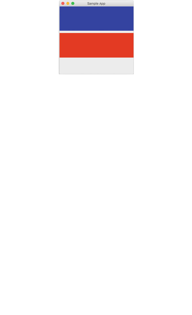
The program that generated this GUI is given below:

import wx

class SampleFrame(wx.Frame):

def __init__(self):

super().__init__(parent=None,

title='Sample App',

size=(300, 300))

# Set up the first Panel to be at position 1, 1

# (The default) and of size 300 by 100

# with a blue background

self.panel1 = wx.Panel(self)

self.panel1.SetSize(300, 100)

self.panel1.SetBackgroundColour(wx.Colour(0, 0, 255))

# Set up the second Panel to be at position 1, 110

# and of size 300 by 100 with a red background

self.panel2 = wx.Panel(self)

self.panel2.SetSize(1, 110, 300, 100)

self.panel2.SetBackgroundColour(wx.Colour(255, 0, 0))

class MainApp(wx.App):

def OnInit(self):

""" Initialise the main GUI Application"""

frame = SampleFrame()

frame.Show()

return True

# Run the GUI application

pp = MainApp()

pp.MainLoop()

8.3 Window Classes 79

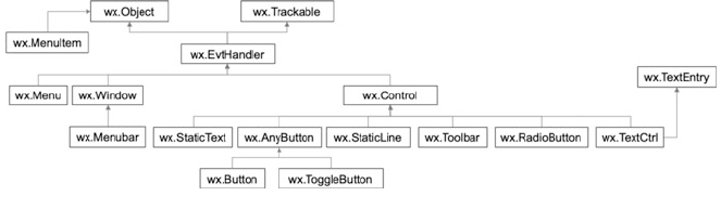
The SampleFrame is a subclass of the wx.Frame class; it thus inherits all of

the functionality of a Top Level Frame (window). Within the __init__()

method of the SampleFrame the super classes __init__() method is called.

This is used to set the size of the Frame and to give the Frame a title. Note that the

Frame also indicates that it does not have a parent window.

When the Panel is created it is necessary to specify the window (or in this case

Frame) within which it will be displayed. This is a common pattern within

wxPython.

Also note that the SetSize method of the Panel class also allows the position

to be speciﬁed and that the Colour class is the wxPython Colour class.

8.4 Widget/Control Classes

Although there are very many widgets/controls available to the developer, the most

commonly used include:

• wx.Button/wx.ToggleButton/wx.RadioButton These are widgets

that provide button like behaviour within a GUI.

• wx.TextCtrl This widget allows text to be displayed and edited. I can be a

single line or multiple line widget depending upon conﬁguration.

• wx.StaticTex t Used to display one or more lines of read-only text. In many

libraries this widgets is known as a label.

• wx.StaticLin e A line used in dialogs to separate groups of widgets. The

line may be vertical or horizontal.

• wx.ListBox This widget is used to allow a user to select one option from a

list of options.

• wx.MenuBar/wx.Menu/wx.MenuItem. The components that can be used to

construct a set of menus for a User Interface.

• wx.ToolBar This widget is used to display a bar of buttons and/or other

widgets usually placed below the menubar in a wx.Frame.

The inheritance hierarchy of these widgets is given below. Note that they all

inherit from the class Control (hence why they are often referred to as Controls

as well as Widgets or GUI components).

80 8 The wxPython GUI Library

Whenever a widget is created it is necessary to provide the container window

class that will hold it, such as a Frame or a Panel, for example:

In this code snipp et a wx.Button is being created that will have a label ‘Enter’

and will be displayed within the given Panel.

8.5 Dialogs

The generic wx.Dialog class can be used to build any custom dialog you require.

It can be used to create modal and modeless dialogs:

• A modal dialog blocks program ﬂow and user input on other windows until it is

dismissed.

• A modeless dialog behaves more like a frame in that program ﬂow continues,

and input in other windows is still possible.

• The wx.Dialog class provides two versions of the show method to support

modal and modeless dialogs. The ShowModal() method is used to display a

modal dialog, while the Show() is used to show a modeless dialog.

As well as the generic wx.Dialog class, the wxPython library provides numerous

prebuilt dialogs for common situations. These pre built dialogs include:

• wx.ColourDia log This class is used to generat e a colour chooser dialog.

• wx.DirDialog This class provides a directory chooser dialog.

• wx.FileDialo g This class provi des a ﬁle chooser dialog.

• wx.FontDialo g This class provi des a font chooser dialog.

• wx.MessageDi alog This class can be used to generat e a single or multi-line

message or information dialog. It can support Yes, No and Cancel options. It

can be used for generic messages or for error messages.

• wx.MultiChoi ceDialog This dialog can be used to display a lit of strings

and allows the user to select one or more values for the list.

• wx.PasswordE ntryDialog This class represents a dialog that allows a

user to enter a one-line password string from the user.

• wx.ProgressD ialog If supported by the GUI platform, then this class will

provide the platforms native progress dialog, otherwise it will use the pure

Python wx.GenericPr ogressDialog. The wx.

GenericProgr essDialog shows a short message and a progress bar.

• wx.TextEntry Dialog This class provides a dialog that requests a one-line

text string from the user.

enter_button = wx.Button(panel, label='Enter')

8.4 Widget/Control Classes 81

Most of the dialogs that return a value follow the same pattern. This pattern

returns a value from the ShowModel() method that indicates if the user selected

OK or CANCEL (using the return value wx.ID_OK or wx.ID_CANCEL). The

selected/entered value can then be obtained from a suitable get method such as

GetColourData() for the ColourDialog or GetPath() for the

DirDialog.

8.6 Arranging Widgets Within a Container

Widgets can be located within a window using speciﬁc coordinates (such as 10

pixels down and 5 pixels across). However, this can be a problem if you are

considering cross platform applications, this is because how a button is rendered

(drawn) on a Mac is different to Windows and different again from the windowing

systems on Linux/Unix etc.

This means that different amount of spacing must be given on different plat-

forms. In addition the fonts used with text boxes and labels differ between different

platforms also requiring differences in the layout of widgets.

To overcome this wxPython provides Sizers. Sizers work with a container such

as a Frame or a Panel to determine how the contained widgets should be laid out.

Widgets are added to a sizer which is then set onto a container such as a Panel.

A Sizer is thus an object which works with a container and the host windowing

platform to determine the best way to display the objects in the window. The

developer does not need to worry about what happens if a user resizes a window or

if the program is executed on a different windowing platform.

Sizers therefore help to produce portable, presentable user interfaces. In fact one

Sizer can be placed within another Sizer to create complex component layouts.

There are several sizers available including:

• wx.BoxSizer This sizer can be used to place several widgets into a row or

column organisation depending upon the orientation. When the BoxSizer is

created the orientation can be speciﬁed using wx.VERTICAL or wx,

HORIZONTAL.

• wx.GridSizer This sizer lays widgets out in a two dimensional grid. Each

cell within the grid has the same size. When the GridSizer object is created it

is possible to specify the number of rows and columns the grid has. It is also

possible to specify the spacing between the cells both horizontally and

vertically.

• wx.FlexGridS izer This sizer is a slightly more ﬂexible version of the

GridSizer. In this version not all columns and rows need to be the same size

(although all cells in the same column are the same width and all cells in the

same row are the same height).

82 8 The wxPython GUI Library

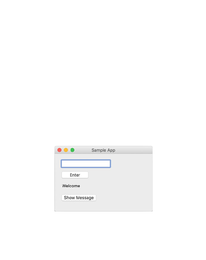
• wx.GridBagSi zer is the most ﬂexible sizer. It allows widgets to be posi-

tioned relative to the grid and also allows widgets to span multiple rows and/or

columns.

To use a Sizer it must ﬁrst be instantiated. When widgets are created they should

be added to the sizer and then the sizer should be set on the container.

For example, the following code uses a GridSizer used with a Panel to

layout out four widgets comprised of two buttons, a StaticText label and a

TextCtrl input ﬁeld:

The resulting display is shown below:

# Create the panel

panel = wx.Panel(self)

# Create the sizer to use with 4 rows and 1 column

# And 5 spacing around each cell

grid = wx.GridSizer(4, 1, 5, 5)

# Create the widgets

text = wx.TextCtrl(panel, size=(150, -1))

enter_button = wx.Button(panel, label='Enter')

label = wx.StaticText(panel,label='Welcome')

message_button = wx.Button(panel, label='Show Message')

# Add the widgets to the grid sizer

grid.AddMany([text, enter_button, label, message_button])

# Set the sizer on the panel

panel.SetSizer(grid)

8.6 Arranging Widgets Within a Container 83

8.7 Drawing Graphics

In earlier chapters we looked at the Turtle graphics API for generating vector and

raster graphics in Python.

The wxPython library provides its own facilities for generating cross platform

graphic displays using lines, squares, circles, text etc. This is provided via the

Device Context.

A Device Context (often shortened to just DC) is an object on which graphics

and text can be drawn.

It is intended to allow different output devices to all have a common graphics

API (also known as the GDI or Graphics Devi ce Interface). Speciﬁc device contexts

can be instantiate depending on whether the program is to use a window on a

computer screen or some other output medium (such as a printer).

There are several Device Context types available such as wx.WindowDC, wx.

PaintDC and wx.ClientDC:

• The wx.WindowDC is used if we want to paint on the whole window

(Windows only). This includes window decorations.

• The wx.ClientDC is used to draw on the client area of a window. The client

area is the area of a window without its decorations (title and border).

• The wx.PaintDC is used to draw on the client area as well but is intended to

support the window refresh paint event handling mechanism.

Note that the wx.PaintDC should be used only from a wx.PaintEvent

handler while the wx.ClientDC should never be used from a wx.PaintEvent

handler.

Whichever Device Context is used, they all suppor t a similar set of methods that

are used to generate graphics, such as:

• DrawCircle (x, y, radius) Draws a circle with the given centre and

radius.

• DrawEllipse (x, y, width, height) Draws an ellipse contained in the

rectangle speciﬁed either with the given top left corner and the given size or

directly.

• DrawPoint (x, y) Draws a point using the color of the current pen.

• DrawRectangl e (x, y, width, height) Dra ws a rectangle with the

given corner coordinate and size.

• DrawText (text, x, y) Draws a text string at the speciﬁed point, using the

current text font, and the current text foreground and background colours.

• DrawLine (pt1, pt2)/DrawLine (x1, y1, x2, y2) This method

draws a line from the ﬁrst point to the second.

It is also important to understand when the device context is refreshed/redrawn.

For example, if you resize a window, maximise it, minimise it, move it, or modify

its contents the window is redrawn. This generates an event, a PaintEvent.

You can bind a method to the Paint Event (usi ng wx.EVT_P AINT) that can

be called each time the window is refreshed.

84 8 The wxPython GUI Library

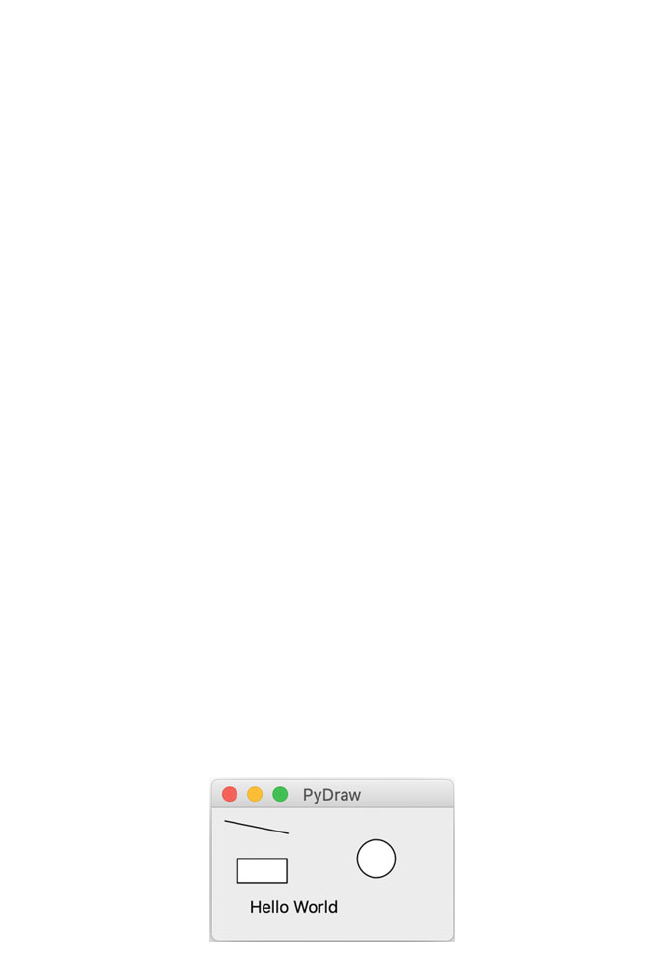
This method can be used to draw whatever the contents of the window shoul d

be. If you do not redraw the contents of the device context in such a method than

whatever you previously drew will display when the window is refreshed.

The following simple program illustrates the use of some of the Draw methods

listed above and how a method can be bound to the paint event so that the display is

refreshed appropriately when using a device context:

When this program is run the following display is generated:

import wx

class DrawingFrame(wx.Frame):

def __init__(self, title):

super().__init__(None,

title=title,

size=(300, 200))

self.Bind(wx.EVT_PAINT, self.on_paint)

def on_paint(self, event):

"""set up the device context (DC) for painting"""

dc = wx.PaintDC(self)

dc.DrawLine(10, 10, 60, 20)

dc.DrawRectangle(20, 40, 40, 20)

dc.DrawText("Hello World", 30, 70)

dc.DrawCircle(130, 40, radius=15)

class GraphicApp(wx.App):

def OnInit(self):

""" Initialise the GUI display"""

frame = DrawingFrame(title='PyDraw')

frame.Show()

return True

# Run the GUI application

app = GraphicApp()

app.MainLoop()

8.7 Drawing Graphics 85

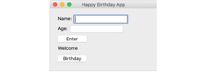
8.8 Online Resources

There are numerous online references that support the development of GUIs and of

Python GUIs in particular, including:

•

https://docs.wxpython. org for documentation on wxPython.

•

https://www.wxpython.org wxPython home page.

•

https://www.wxwidgets.org For information on the underlying wxWidgets

Cross platform GUI library.

8.9 Exercises

8.9.1 Simple GUI Application

In this exercise you will implement your own simple GUI application.

The application should generate the display for a simple UI. An example of the

user interface is given below:

Notice that we have added a label to the input ﬁelds for name and age; you can

manage their display using a nested panel.

In the next chapter we will add event handling to this application so that the

application can respond to button clicks etc.

86 8 The wxPython GUI Library

Chapter 9

Events in wxPython User Interfaces

9.1 Event Handling

Events are an integral part of any GUI; they represent user interactions with the

interface such as c licking on a button, entering text into a ﬁeld, selecting a menu

option etc.

The main event loop listens for an event; when one occurs it processes that event

(which usually results in a function or method being called) and then waits for the

next event to happen. This loop is initiated in wxPython via the call to the

MainLoop() method on the wx.App object.

This raises the question ‘what is an Event?’. An event object is a piece of

information representing some interaction that occurred typically with the GUI

(although an event can be generated by anything). An event is processed by an

Event Handler. This is a method or function that is called when the event occurs.

The event is passed to the handler as a parameter. An Event Binder is used to bind

an event to an event handler.

9.2 Event Deﬁnitions

It is useful to summarise the deﬁnitions around events as the terminology used can

be confusing and is very similar:

• Event represents information from the underlying GUI framework that

describes something that has happened and any associated data. The speciﬁc

data available will differ depending on what has occurred. For example, if a

window has been moved then the associated data will relate to the window’s

new location. Where as a CommandEvent generated by a selection action from

a ListBox provides the item index for the selection.

J. Hunt, Advanced Guide to Python 3 Programming,

Undergraduate Topics in Computer Science,

https://doi.org/10.1007/978-3-030-25943-3_9

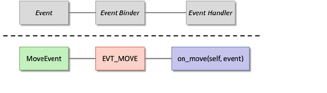
• Event Loop the main processing loop of the GUI that waits for an event to

occur. When an event occurs the associated event handler is called.

• Event Handlers these are methods (or functions) that are called when an event

occurs.

• Event Binders associate a type of event with an event handler. There are

different event binders for different types of event. For example, the event binder

associated with the wx.MoveEvent is named wx.EVT_MOVE.

The relationship between the Event, the Event Handler via the Event Binder is

illustrated below:

The top three boxes illustrate the concepts while the lower 3 boxes provide a

concrete example of binding a Move_Event to an on_move() method via the

EVT_MOVE binder.

9.3 Types of Events

There are numerous different types of event incl uding:

• wx.CloseEven t used to indicate that a Frame or Dialog has been closed. The

event binder for this event is named wx.EVT_CLOSE.

• wx.CommandEv ent used with widgets such as buttons, list boxes, menu

items, radio buttons, scrollbars, sliders etc. Depending upon the type of widget

that generated the event different infor mation may be provided. For example, for

a Button a CommandEvent indicates that a button has been clicked where as

for a ListBox it indicates that an option has been selected, etc. Different event

binders are used for different event situations. For example, to bind a command

event to a event handler for a button then the wx.EVT_BUTTON binder is used;

while for a ListBox a wx.EVT_LISTBOX binder can be used.

• wx.FocusEven t This event is sent when a window’s focus changes (loses or

gains focus). You can pick up a window gaining focus using the wx.

EVT_SET_FOCU S event binder. The wx.EVT_KILL_FOCUS is used to bind

an event handler that will be called when a window loses focus.

88 9 Events in wxPython User Interfaces

• wx.KeyEvent This event contains information relating to a key press or

release.

• wx.MaximizeE vent This event is generated when a top level window is

maximised.

• wx.MenuEvent This event is used for menu oriented actions such as the menu

being opened or closed; however it should be noted that this event is not used

when a menu item is selected (MenuItems generate CommandEvents).

• wx.MouseEven t This event class contains information about the events

generated by the mouse: this includes information on which mouse button was

pressed (and released) and whether the mouse was double clicked etc.

• wx.WindowCre ateEvent This event is sent just after the actual window is

created.

• wx.WindowDes toryedEvent This event is sent as early as possible during

the window destruction process.

9.4 Binding an Event to an Event Handler

An event is bound to an Event Handler using the Bind() method of an event

generating object (such as a button, ﬁeld, menu item etc.) via a named Event

Binder.

For example:

button.Bind(wx.EVT_BUTTON, self.event_handler_method)

9.5 Implementing Event Handling

There are four steps involved in implementing event handling for a widget or

window, these are:

1. Identify the event of interest. Many widgets will generate different events in

different situations; it may therefore be necessary to determine which event you

are interested in.

2. Find the correct Event Binder name, e.g. wx.EVT_CLOSE, wx.EVT_MOVE

or wx.EVT_BUTTON etc. Again you may ﬁnd that the widget you are inter-

ested in supports numerous different event binders which may be used in dif-

ferent situations (even for the same event).

3. Implement an event handler (i.e. a suitable method or function) that will be

called when the event occurs. The event handler will be supplied with the event

object.

4. Bind the Event to the Event Handler via the Binder Name using the Bind()

method of the widget or window.

9.3 Types of Events 89

To illustrate this we will use a simple example.

We will write a very simple event handlin g application. This application will

have a Frame containing a Panel. The Panel will contain a label using the wx.

StaticText class.

We will deﬁne an event handler called on_mouse_click() that will move

the StaticText label to the current mouse location when the left mouse button is

pressed. This means that we can move the label around the screen.

To do this we ﬁrst need to determine the widget that will be used to generate the

event. In this case it is the panel that contains the text label. Having done this we

can look at the Panel class to see what events and Event Bindings it supports. It

turns out that the Panel class only directly deﬁnes support for

NavigationKeyEvents. This is not actually what we want; however the

Panel class extends the Window class.

The Window class supports numerous event bindings, from those associated

with setting the focus (wx.EVT_SET_FOCUS and wx.EVT_KILL_FOCUS)to

key presses (wx.EVT_KEY_DOWN and wx.EVT_KEY_UP) as well as mouse

events. There are however numerous different mouse event bindings. These allow

left, middle and right mouse button clicks to be picked up, down clicks to be

identiﬁed, situations such as the mouse entering or leaving the window etc.

However, the binding we are inte rested in for a MouseEvent is the wx.

EVT_LEFT_DOWN binding; this picks up on the MoueEvent when the left mouse

button is pressed (there is also the wx.EVT_LEFT_UP binding which can be used

to pick up an event that occurs when the left mouse button is released).

We now know that we need to bind the on_mouse_click() event handler to

the MouseEvent via the wx.EVT_LEFT_DOWN event binder, for example:

self.panel.Bind(wx.EVT_LEFT_DOWN, self.on_mouse_click)

All event handler methods takes two parameters, self and the mouse event.

Thus the signature of the on_mouse_click() method is:

def on_mouse_click(self, mouse_event):

The mouse event object has numerous methods deﬁned that allow information

about the mouse to be obtained such as the number of mouse clicks involved

(GetClickCount()), which button was pressed (GetButton()) and the

current mouse position within the containing widget or window (GetPosition

()). We can therefore use this last method to obtain the current mouse location and

then use the SetPosition(x, y) method on the StaticText object to set its

position.

The end result is the program shown below:

90 9 Events in wxPython User Interfaces

import wx

class WelcomeFrame(wx.Frame):

""" The Main Window / Frame of the application """

def __init__(self):

super().__init__(parent=None,

title='Sample App',

size=(300, 200))

# Set up panel within the frame and text label

self.panel = wx.Panel(self)

self.text = wx.StaticText(self.panel,

label='Hello')

# Bind the on_mouse_click method to the

# Mouse Event via the

# left mouse click binder

self.panel.Bind(wx.EVT_LEFT_DOWN,

self.on_mouse_click)

def on_mouse_click(self, mouse_event):

""" When the left mouse button is clicked

This method is called. It will obtain

the current mouse coordinates, and

reposition the text label

to this position. """

x, y = mouse_event.GetPosition()

print(x, y)

self.text.SetPosition(wx.Point(x, y))

class MainApp(wx.App):

def OnInit(self):

""" Initialise the main GUI Application"""

frame = WelcomeFrame()

frame.Show()

# Indicate that processing should continue

return True

# Run the GUI application

app = MainApp()

app.MainLoop()

9.5 Implementing Event Handling 91

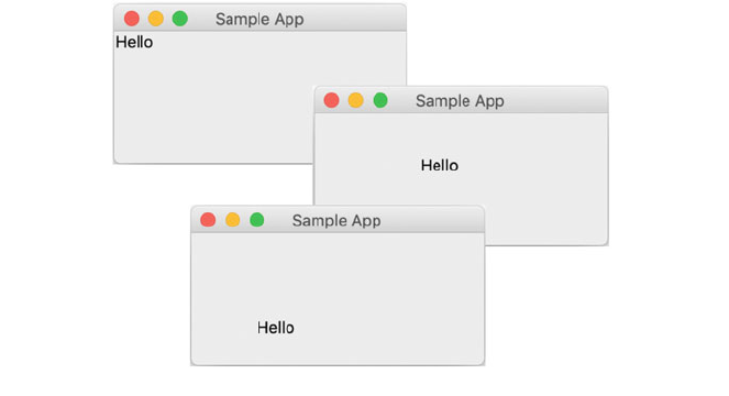
When this program is run; the window is displayed with the ‘Hello’

StaticText label in the top left hand corner of the Frame (actually it is added to

the Panel, however the Panel ﬁlls the Frame in this example). If the user then

clicks the left mouse button anywhere within the Frame then the ‘Hello’ label jumps

to that location.

This is shown below for the initial setup and then for two locations within the

window.

9.6 An Interactive wxPython GUI

An example of a slightly larger GUI application, that brings together many of the

ideas presented in this chapter, is given below.

In this application we have a text input ﬁeld (a wx.TextCtrl) that allows a

user to enter their name. When they click on the Enter button (wx.Button ) the

welcome label (a wx.StaticText) is updated with their name. The ‘Show

Message’ button is used to display a wx.MessageDialog which will also

contain their name.

The initial display is shown below for both a Mac and a Windows PC, note that

the default background colour for a Frame is different on a Windows PC than on a

Mac and thus although the GUI runs on both plat forms, the look differs between the

two:

92 9 Events in wxPython User Interfaces

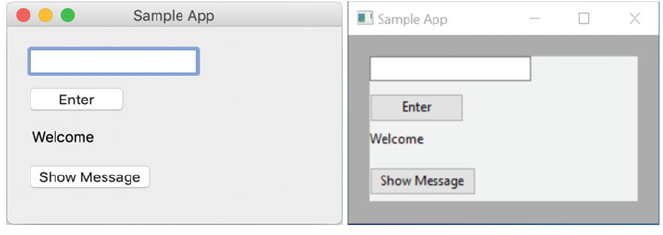
The code used to implement this GUI application is given below:

import wx

class HelloFrame(wx.Frame):

def __init__(self, title):

super().__init__(None, title=title, size=(300, 200))

self.name = '<unknown>’

# Create the BoxSizer to use for the Frame

vertical_box_sizer = wx.BoxSizer(wx.VERTICAL)

self.SetSizer(vertical_box_sizer)

# Create the panel to contain the widgets

panel = wx.Panel(self)

# Add the Panel to the Frames Sizer

vertical_box_sizer.Add(panel,

wx.ID_ANY,

wx.EXPAND | wx.ALL,

20)

# Create the GridSizer to use with the Panel

grid = wx.GridSizer(4, 1, 5, 5)

# Set up the input field

self.text = wx.TextCtrl(panel, size=(150, -1))

9.6 An Interactive wxPython GUI 93

# Set the sizer on the panel

panel.SetSizer(grid)

# Centre the Frame on the Computer Screen

self.Centre()

def show_message(self, event):

""" Event Handler to display the Message Dialog

using the current value of the name attribute. """

dialog = wx.MessageDialog(None,

message=’Welcome To Python ' + self.name,

caption=’Hello',

style=wx.OK)

dialog.ShowModal()

def set_name(self, event):

""" Event Handler for the Enter button.

Retrieves the text entered into the input field

and sets the self.name attribute. This is then

used to set the text label """

self.name = self.text.GetLineText(0)

self.label.SetLabelText('Welcome ' + self.name)

# Now configure the enter button

enter_button = wx.Button(panel, label='Enter')

enter_button.Bind(wx.EVT_BUTTON, self.set_name)

# Next set up the text label

self.label = wx.StaticText(panel,

label='Welcome',

style=wx.ALIGN_LEFT)

# Now configure the Show Message button

message_button = wx.Button(panel, label='Show Message')

message_button.Bind(wx.EVT_BUTTON, self.show_message)

# Add the widgets to the grid sizer to handle layout

grid.AddMany([self.text,

enter_button,

self.label,

message_button])

94 9 Events in wxPython User Interfaces

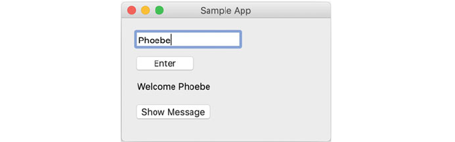
class MainApp(wx.App):

def OnInit(self):

""" Initialise the GUI display"""

frame = HelloFrame(title='Sample App')

frame.Show()

# Indicate whether processing should continue or no

return True

def OnExit(self):

""" Executes when the GUI application shuts down"""

print('Goodbye')

# Need to indicate success or failure

return True

# Run the GUI application

app = MainApp()

app.MainLoop()

If the user enters their name in the top TextCtrl ﬁeld, for example ‘Phoebe’, then

when they click on the ‘Enter’ button the welcome label changes to ‘Welcome

Phoebe’:

If they now click on the ‘Show Message’ button then the wx.

MessageDialog (a speciﬁc type of wx.Dialog) will display a welcome

message to Phoebe:

9.6 An Interactive wxPython GUI 95

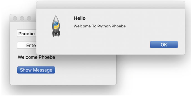
9.7 Online Resources

There are numerous online references that support the development of GUIs and of

Python GUIs in particular, including:

•

https://docs.wxpython. org for documentation on wxPython.

•

https://www.wxpython.org wxPython home page.

•

https://www.wxwidgets.org For information on the underlying wxWidgets

Cross platform GUI library.

9.8 Exercises

9.8.1 Simple GUI Application

This exercise builds on the GUI you created in the last chapter.

The application should allow a user to enter their name and age. You will need to

check that the value entered into the age ﬁeld is a numeric value (for example using

isnumeric()). If the value is not a number then an error mess age dialog should

be displayed.

96 9 Events in wxPython User Interfaces

A button should be provided labelled ‘Birthday’; when clicked it should

increment the age by one and display a Happy Birthday message. The age should be

updated within the GUI.

An example of the user interface you created in the last chapter is given below:

As an example, the user might enter their name and age as shown below:

When the user clicks on the ‘birthday’ button then the Happy Birthday message

dialog is displayed:

9.8 Exercises 97

9.8.2 GUI Interface to a Tic Tac Toe Game

The aim of this exercise is to implement a simple Tic Tac Toe game. The game

should allow two users to play interactive using the same mouse. The ﬁrst user will

have play as the ‘X’ player and the second user as the ‘0’ player.

When each user selects a button you can set the label for the button to their

symbol.

You will need two check after each move to see if someone has won (or if the

game is a draw).

You will still need an internal representation of the grid so that you can deter-

mine who, if anyone, has won.

An example of how the GUI for the TicTacToe game might look is given below:

You can also add dialogs to obtain the players names and to notify them who

won or whether there was a draw.

98 9 Events in wxPython User Interfaces

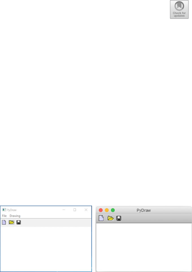
Chapter 10

PyDraw wxPython Example Application

10.1 Introduction

This chapter builds on the GUI library presented in the last tw o chapters to illustrate

how a larger application can be built. It presents a case study of a drawing tool akin

to a tool such as Visio etc.

10.2 The PyDraw Application

The PyDraw application allows a user to draw diagrams using square s, circles, lines

and text. At present there is no select, resize, reposition or delete option available

(although these could be added if required). PyDraw is implemented using the

wxPython set of components as deﬁned in version 4.0.6.

When a user starts the PyDraw application, they see the interface shown above

(for both the Microsoft Windows and Apple Mac operating systems). Depending on

J. Hunt, Advanced Guide to Python 3 Programming,

Undergraduate Topics in Computer Science,

https://doi.org/10.1007/978-3-030-25943-3_10

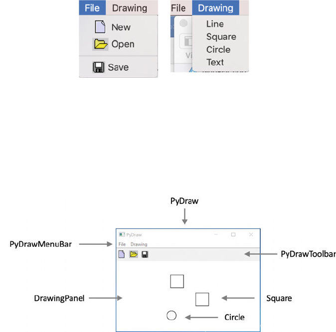
the operating system it ha s a menu bar across the top (on a Mac this menu bar is at

the Top of the Mac display), a tool bar below the menu bar and a scrollable drawing

area below that.

The ﬁrst button on the tool bar clears the drawing area. The second and third

buttons are only implemented so that they print out a message into the Python

console, but are intended to allow a user to load and save drawings.

The tool bar buttons are duplicated on the menus deﬁned for the application,

along with a drawing tool selection menu, as shown below:

10.3 The Structure of the Application

The user interface created for the PyDraw application is made up of a number of

elements (see below): the PyDrawMenuBar, the PyDrawToolbar containing a

sequence of buttons across the top of the window, the drawing panel, and the

window frame (implemented by the PyDrawFrame class).

The following diagram shows the same information as that presented above, but

as a containment hierarchy, this means that the diagram illustrates how one object is

contained within another. The lower level objects are contained within the higher

level objects.

100 10 PyDraw wxPython Example Application

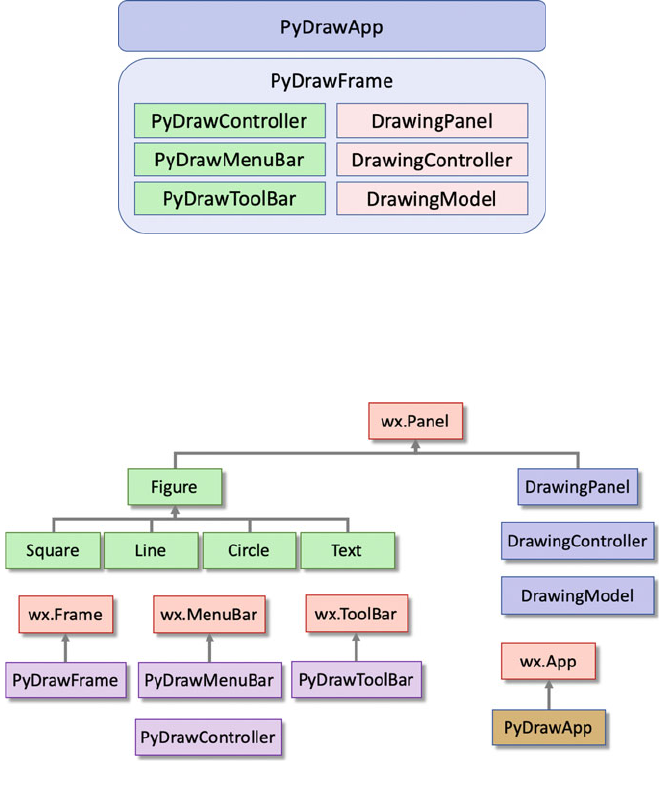
It is important to visualize this as the majority of wxPython interfaces are built

up in this way, using containers and sizers.

The inheritance structure between the classes used in the PyDraw application is

illustrated below. This class hierarchy is typical of an application which incorpo-

rates user interface features with graphical elements.

10.3.1 Model, View and Controller Archit ecture

The application adopts the well established Model-View-Controller (or MVC)

design pattern for separating out the responsibilities between the view element (e.g.

the Frame or Panel), the control element (for handling user input) and the model

element (which holds the data to be displayed).

This separation of concerns is not a new idea and allows the construction of GUI

applications that mirror the Model-View-Controller architecture. The intention of

the MVC architecture is the separation of the user display, from the control of user

input, from the underlying information model as illustrated below.

10.3 The Structure of the Application 101

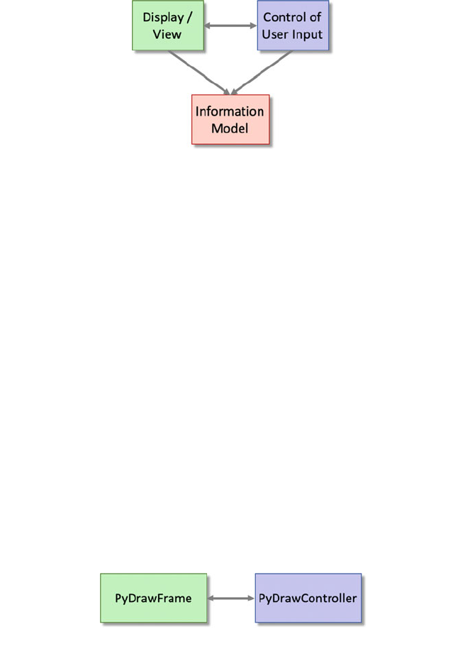
There are a number of reasons why this separation is useful:

• reusability of application and/or user interface components,

• ability to develop the application and user interface separately,

• ability to inherit from different parts of the class hierarchy.

• ability to deﬁne control style classes which provide common features separately

from how these features may be displayed.

This means that different interfaces can be used with the same application,

without the application knowing about it. It also means that any part of the system

can be changed without affectin g the operation of the other. For example, the way

that the graphical interface (the look) displays the information could be changed

without modifying the actual application or how input is handled (the feel). Indeed

the application need not know what type of interface is currently connected to it at

all.

10.3.2 PyDraw MVC Architecture

The MVC structure of the PyDraw application has a top level controller class

PyDrawController and a top level view class the PyDrawFrame (there is no

model as the top level MVC triad does not hold any expli cit data itself). This is

shown below:

At the next level down there is another MVC structure; this time for the drawing

element of the application. There is a DrawingController, with a

DrawingModel and a DrawingPanel (the view) as illustrated below:

102 10 PyDraw wxPython Example Application

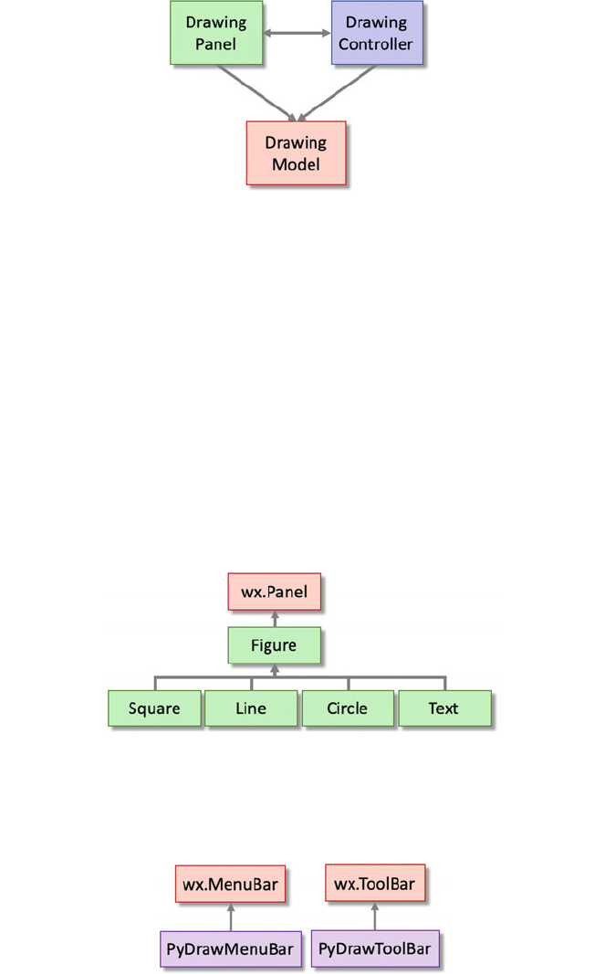
The DrawingModel, DrawingPanel and DrawingController classes

exhibit the classic MVC structure. The view and the controller classes

(DrawingPanel and DrawingController) know about each other and the

drawing model, whereas the DrawingModel knows nothing about the view or the

controller. The view is notiﬁed of changes in the drawing through the paint event.

10.3.3 Additional Classes

There are also four types of drawing object (of Figure): Circle, Line, Square

and Text ﬁgures. The only difference between these classes is what is drawn on

the graphic device context within the on_paint() method. The Figure class,

from which they all inherit, deﬁnes the common attributes used by all objects within

a Drawing (e.g. point representing an x and y location and size).

The PyDrawFrame class also uses a PyDrawMenuBar and a

PyDrawToolBar class. The ﬁrst of these extends the wx.MenuBar with menu

items for use within the PyDraw application. In turn the PyDrawToolBar extends

the wx.ToolBar and provides icons for use in PyDraw.

10.3 The Structure of the Application 103

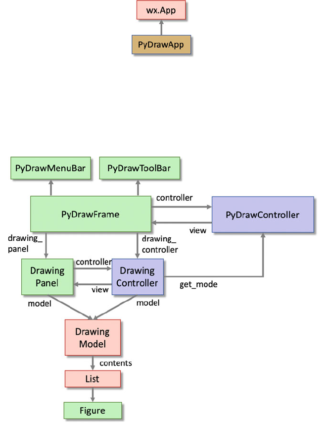
The ﬁnal class is the PyDrawApp class that extends the wx.App class.

10.3.4 Object Relationships

However, the inher itance hierarchy is only part of the story for any object oriented

application. The following ﬁgure illustrates how the objects relate to one another

within the working application.

The PyDrawFrame is responsible for setting up the controller and the

DrawingPanel.

The PyDrawController is responsible for handling menu and tool bar user

interactions.

This separates graphical elements from the behaviour triggered by the user.

104 10 PyDraw wxPython Example Application

The DrawingPanel is responsible le for displaying any ﬁgures held by the

DrawingModel. The DrawingController manages all user interactions with

the DrawingPanel including adding ﬁgures and clearing all ﬁgures from the

model. The DrawingModel holds list of ﬁgures to be displayed.

10.4 The Interactions Between Objects

We have now examined the physical structure of the application but not how the

objects within that application interact.

In many situations this can be extracted from the source code of the application

(with varying degrees of difﬁculty). However, in the case of an application such as

PyDraw, which is made up of a number of different inte racting components, it is

useful to describe the system interactions explicitly.

The diagrams illustrating the interactions between the objects use the following

conventions:

• a solid arrow indicates a message send,

• a square box indicates a class,

• a name in brackets indicates the type of instance,

• numbers indicate the sequence of message sends.

These diagrams are based on the collaboration diagrams found in the UML

(Uniﬁed Modelling Language) notation.

10.4.1 The PyDrawApp

When the PyDrawApp is instantiated the PyDrawFrame in created and displayed

using the OnInit() method. The MainLoop() method is then invoked. This is

shown below:

def OnInit(self):

""" Initialise the GUI display"""

frame = PyDrawFrame(title='PyDraw')

frame.Show()

return True

# Run the GUI application

app = PyDrawApp()

app.MainLoop()

class PyDrawApp(wx.App):

10.3 The Structure of the Application 105

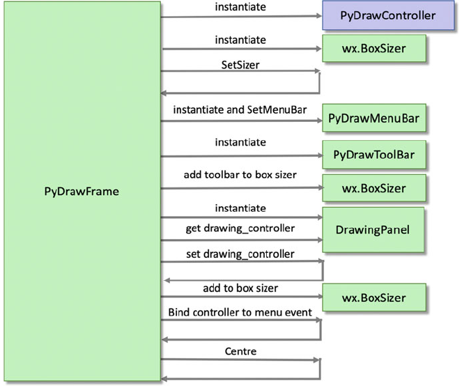
10.4.2 The PyDrawFrame Constructor

The PyDrawFrame constructor method sets up the main display of the UI

application and also initialises the controllers and drawing elements. This is shown

below using a collaboration diagram:

The PyDrawFrame constructor sets up the environment for the application. It

creates the top level PyDr awController. It creat es the DrawingPanel and

initialises the display layout. It initialises the menu bar and tool bar. It binds the

controllers menu handler to the menus and centers itself.

10.4.3 Changing the Application Mode

One interesting thing to note is what happens when the user selects an option from

the Drawing menu. This allows the mode to be changed to a square, circle, line or

text. The interactions involved are shown below for the situation where a user

selects the ‘Circl e ’ menu item on the Drawing menu (using a collaboration

diagram):

106 10 PyDraw wxPython Example Application

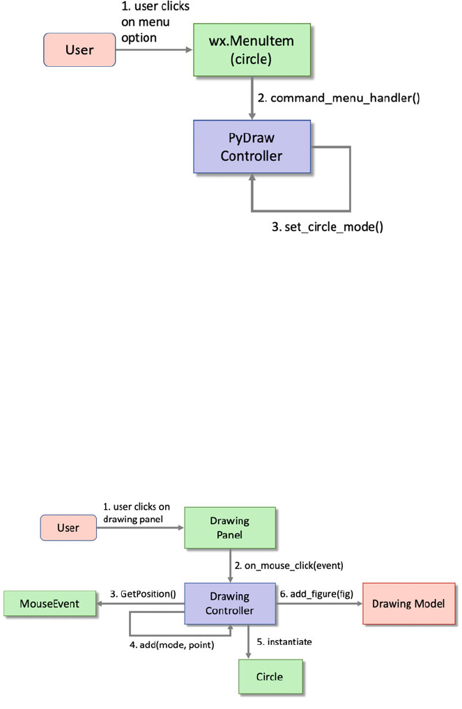
When the user selects one of the menu items the command_menu_handler

() method of the PyDrawController is invoked. This method determines

which menu item has been selected; it then calls an appropriate setter method (such

as set_circle_mode() or set_line_mode() etc.). These methods set the

mode attribute of the controller to an appropriate value.

10.4.4 Adding a Graphic Object

A user adds a graphic object to the drawing displayed by the DrawingPanel by

pressing the mouse button.

When the user clicks on the drawing panel, the DrawingController

responds as shown below:

10.4 The Interactions Between Objects 107

The above illustrates what happens when the user presses and releases a mouse

button over the drawing panel, to create a new ﬁgure.

When the user presses the mouse button, a mouse clicked message is sent to the

DrawingController, which decides what action to perform in response (see

above). In PyDraw, it obtains the cursor point at which the event was generated by

calling the GetPosition() method on the mouse_event.

The controller then calls its own add() method passing in the current mode and

the current mouse location. The controller obtains the current mode (from the

PyDrawController using the method callback provided when the

DrawingController is instantiated) and adds the appropriate type of ﬁgure to

the DrawingModel.

The add() method then adds a new ﬁgure to the drawing model based on the

speciﬁed mode.

10.5 The Classes

This section presents the classes in the PyDraw application. As these classes build

on concepts already presented in the last few chapters, they shall be presented in

their entirety with comments highlighting speciﬁc points of their implementations.

Note that the code imports the wx module from the wxPython library, e.g.

import wx

10.5.1 The PyDrawConstants Class

The purpose of this class is to provide a set of constants that can be referenced in

the remainder of the application. It is used to provide constants for the IDs used

with menu items and toolbar tools. It also provides constants used to represent the

current mode (to indicate whether a line, square, circle or test should be added to the

display).

class PyDrawConstants:

LINE_ID = 100

SQUARE_ID = 102

CIRCLE_ID = 103

TEXT_ID = 104

SQUARE_MODE = 'square'

LINE_MODE = 'line'

CIRCLE_MODE = 'circle'

TEXT

MODE = 'Text'

108 10 PyDraw wxPython Example Application

10.5.2 The PyDrawFrame Class

The PyDrawFrame class provides the main window for the application. Note that

due to the separation of concerns introduced via the MVC architecture, the view

class is only concerned with the layout of the components:

class PyDrawFrame(wx.Frame):

""" Main Frame responsible for the

layout of the UI."""

def __init__(self, title):

super().__init__(None,

title=title,

size=(300, 200))

# Set up the controller

self.controller = PyDrawController(self)

# Set up the layout fo the UI

self.vertical_box_sizer = wx.BoxSizer(wx.VERTICAL)

self.SetSizer(self.vertical_box_sizer)

# Set up the menu bar

self.SetMenuBar(PyDrawMenuBar())

# Set up the toolbar

self.vertical_box_sizer.Add(PyDrawToolBar(self),

wx.ID_ANY,

wx.EXPAND | wx.ALL, )

# Setup drawing panel

self.drawing_panel = DrawingPanel(self,

self.controller.get_mode)

self.drawing_controller = self.drawing_panel.controller

# Add the Panel to the Frames Sizer

self.vertical_box_sizer.Add(self.drawing_panel,

wx.ID_ANY,

wx.EXPAND | wx.ALL)

# Set up the command event handling for the menu bar

and tool bar

self.Bind(wx.EVT_MENU,

self.controller.command_menu_handler)

self.Centre()

10.5 The Classes 109

10.5.3 The PyDrawMenuBar Class

The PyDrawMenuBar class is a subclass of the wx.MenuBar class which deﬁnes

the contents of the menu bar for the PyDraw application. It does this by creating two

wx.Menu objects and adding them to the menu bar. Each wx.Menu implements a

drop down menu from the menu bar. To add individual menu items the wx.

MenuItem class is used. These menu items are appended to the menu. The menus

are themselves appended to the menu bar. Note that each menu item has an id that

can be used to identify the source of a command event in an event handle r. This

allows a single event handler to deal with events generated by multiple menu items.

class PyDrawMenuBar(wx.MenuBar):

def __init__(self):

super().__init__()

fileMenu = wx.Menu()

newMenuItem = wx.MenuItem(fileMenu, wx.ID_NEW,

text="New", kind=wx.ITEM_NORMAL)

newMenuItem.SetBitmap(wx.Bitmap("new.gif"))

fileMenu.Append(newMenuItem)

loadMenuItem = wx.MenuItem(fileMenu, wx.ID_OPEN,

text="Open", kind=wx.ITEM_NORMAL)

loadMenuItem.SetBitmap(wx.Bitmap("load.gif"))

fileMenu.Append(loadMenuItem)

fileMenu.AppendSeparator()

saveMenuItem = wx.MenuItem(fileMenu, wx.ID_SAVE,

text="Save", kind=wx.ITEM_NORMAL)

saveMenuItem.SetBitmap(wx.Bitmap("save.gif"))

fileMenu.Append(saveMenuItem)

fileMenu.AppendSeparator()

quit = wx.MenuItem(fileMenu, wx.ID_EXIT,

'&Quit\tCtrl+Q')

fileMenu.Append(quit)

self.Append(fileMenu, '&File')

drawingMenu = wx.Menu()

lineMenuItem = wx.MenuItem(drawingMenu,

PyDraw_Constants.LINE_ID, text="Line", kind=wx.ITEM_NORMAL)

drawingMenu.Append(lineMenuItem)

squareMenuItem = wx.MenuItem(drawingMenu,

PyDraw_Constants.SQUARE_ID, text="Square", kind=wx.ITEM_NORMAL)

drawingMenu.Append(squareMenuItem)

circleMenuItem = wx.MenuItem(drawingMenu,

110 10 PyDraw wxPython Example Application

PyDraw_Constants.CIRCLE_ID, text="Circle", kind=wx.ITEM_NORMAL)

drawingMenu.Append(circleMenuItem)

textMenuItem = wx.MenuItem(drawingMenu,

PyDraw_Constants.TEXT_ID, text="Text", kind=wx.ITEM_NORMAL)

drawingMenu.Append(textMenuItem)

self.Append(drawingMenu, '&Drawing')

10.5.4 The PyDrawToolBar Class

The DrawToolBar class is a subclass of wx.ToolBar. The classes constructor

initialises three tools that are displayed within the toolbar. The Realize()

method is used to ensure that the tools are rendered appropriately. Note that

appropriate ids have been used to allow an event handler to identify which tools

generated a particular command event. By reusing the same ids for related menu

items and command tools, a single handler can be used to manag e events from both

types of sources.

class PyDrawToolBar(wx.ToolBar):

def __init__(self, parent):

super().__init__(parent)

self.AddTool(toolId=wx.ID_NEW, label="New",

bitmap=wx.Bitmap("new.gif"), shortHelp='Open drawing',

kind=wx.ITEM_NORMAL)

self.AddTool(toolId=wx.ID_OPEN, label="Open",

bitmap=wx.Bitmap("load.gif"), shortHelp='Open drawing',

kind=wx.ITEM_NORMAL)

self.AddTool(toolId=wx.ID_SAVE, label="Save",

bitmap=wx.Bitmap("save.gif"), shortHelp='Save drawing',

kind=wx.ITEM_NORMAL)

self.Realize()

10.5.5 The PyDrawController Class

This class provides the control element of the top level view. It maintains the

current mode and implements a handler that can handle events from menu items

and from the tool bar tools. An id is used to identify each individual menu or tool

which allows a single handler to be registered with the frame.

10.5 The Classes 111

def __init__(self, view):

self.view = view

# Set the initial mode

self.mode = PyDrawConstants.SQUARE_MODE

def set_circle_mode(self):

self.mode = PyDrawConstants.CIRCLE_MODE

def set_line_mode(self):

self.mode = PyDrawConstants.LINE_MODE

def set_square_mode(self):

self.mode = PyDrawConstants.SQUARE_MODE

def set_text_mode(self):

self.mode = PyDrawConstants.TEXT_MODE

def clear_drawing(self):

self.view.drawing_controller.clear()

def get_mode(self):

return self.mode

def command_menu_handler(self, command_event):

id = command_event.GetId()

if id == wx.ID_NEW:

print('Clear the drawing area')

self.clear_drawing()

elif id == wx.ID_OPEN:

print('Open a drawing file')

elif id == wx.ID_SAVE:

print('Save a drawing file')

elif id == wx.ID_EXIT:

print('Quite the application')

self.view.Close()

elif id == PyDrawConstants.LINE_ID:

print('set drawing mode to line')

self.set_line_mode()

elif id == PyDrawConstants.SQUARE_ID:

print('set drawing mode to square')

self.set_square_mode()

elif id == PyDrawConstants.CIRCLE_ID:

print('set drawing mode to circle')

self.set_circle_mode()

elif id == PyDrawConstants.TEXT_ID:

print('set drawing mode to Text')

self.set_text_mode()

else:

rint

(

'Unknown o

tion'

)

class PyDrawController:

112 10 PyDraw wxPython Example Application

10.5.6 The DrawingModel Class

The DrawingModel class has a contents attribute that is used to hold all the

ﬁgures in the drawing. It also provides some convenience metho ds to reset the

contents and to add a ﬁgure to the contents.

class DrawingModel:

def __init__(self):

self.contents = []

def clear_figures(self):

self.contents = []

def add_figure(self, figure):

self.contents.append(figure)

The DrawingModel is a relatively simple model which merely records a set of

graphical ﬁgures in a List. These can be any type of object and can be displayed in

any way as long as they implement the on_paint() method. It is the objects

themselves which determine what they look like when drawn.

10.5.7 The DrawingPanel Class

The DrawingPanel class is a subclass of the wx.Panel class. It provides the

view for the drawing data model. This uses the classical MVC architecture and has

a model (DrawingModel), a view (the DrawingPanel) and a controller (the

DrawingController).

The DrawingPanel instantiates its own DrawingController to handle

mouse events.

It also registers for paint events so that it knows when to refresh the display.

class DrawingPanel(wx.Panel):

def __init__(self, parent, get_mode):

super().__init__(parent, -1)

self.SetBackgroundColour(wx.Colour(255, 255, 255))

self.model = DrawingModel()

self.controller = DrawingController(self, self.model,

get_mode)

self.Bind(wx.EVT_PAINT, self.on_paint)

self.Bind(wx.EVT_LEFT_DOWN,

self.controller.on

mouse

click)

10.5 The Classes 113

def on_paint(self, event):

"""set up the device context (DC) for painting"""

dc = wx.PaintDC(self)

for figure in self.model.contents:

figure.on

paint(dc)

10.5.8 The DrawingController Class

The DrawingController class provides the control class for the top level

MVC architecture used with the DrawingModel (model) and DrawingPanel

(view) classes. In particular it handles the mouse events in the DrawingPanel via the

on_mouse_click() method.

It also deﬁnes an add method that is used to add a ﬁgure to the DrawingModel

(the actual ﬁgure depends on the current mode of the PyDrawController).

A ﬁnal method, the clear() method, removes all ﬁgures from the drawing model

and refreshes the display.

class DrawingController:

def __init__(self, view, model, get_mode):

self.view = view

self.model = model

self.get_mode = get_mode

def on_mouse_click(self, mouse_event):

point = mouse_event.GetPosition()

self.add(self.get_mode(), point)

def add(self, mode, point, size=30):

if mode == PyDrawConstants.SQUARE_MODE:

fig = Square(self.view, point, wx.Size(size, size))

elif mode == PyDrawConstants.CIRCLE_MODE:

fig = Circle(self.view, point, size)

elif mode == PyDrawConstants.TEXT_MODE:

fig = Text(self.view, point, size)

elif mode == PyDrawConstants.LINE_MODE:

fig = Line(self.view, point, size)

self.model.add_figure(fig)

def clear(self):

self.model.clear_figures()

self.view.Refresh()

114 10 PyDraw wxPython Example Application

10.5.9 The Figure Class

The Figure class (an abstract superclass of the Figure class hierarchy) captures

the elements which are common to graphic objects displayed within a drawing. The

point deﬁnes the position of the ﬁgure, while the size attribute deﬁnes the size

of the ﬁgure. Note that the Figure is a subclass of a wx.Panel and thus the

display is constructed from inner panels onto whi ch the various ﬁgure shapes are

drawn.

The Figure class deﬁnes a single abstract method on_paint(dc) that must be

implemented by all concrete subclasses. This method should deﬁne how the shape

is drawn on the drawing panel.

class Figure(wx.Panel):

def __init__(self, parent, id=wx.ID_ANY, pos=None,

size=None, style=wx.TAB_TRAVERSAL):

wx.Panel.__init__(self, parent, id=id, pos=pos,

size=size, style=style)

self.point = pos

self.size = size

@abstractmethod

def on_paint(self, dc):

Pass

10.5.10 The Square Class

This is a subclass of Figure that speciﬁes how to draw a square shape in a

drawing. It implements the on_paint() method inherited from Figure.

class Square(Figure):

def __init__(self, parent, pos, size):

super().__init__(parent=parent, pos=pos, size=size)

def on_paint(self, dc):

dc.DrawRectangle(self.point, self.size)

10.5 The Classes 115

10.5.11 The Circle Class

This is another subclass of Figure. It implements the on_paint() method by

drawing a circle. Note that the shape will be drawn within the panel size deﬁned via

the Figure class (using the call to super). It is therefore necessary to see the circle

to ﬁt within these bounds. This means that the size attribute must be used to generate

an appropriate radius. Also note that the DrawCircle() method of the device

context takes a point that is the centre of the circle so this must also be calculated.

class Circle(Figure):

def __init__(self, parent, pos, size):

super().__init__(parent=parent, pos=pos,

size=wx.Size(size, size))

self.radius = (size - 10) / 2

self.circle_center = wx.Point(self.point.x +

self.radius, self.point.y + self.radius)

def on_paint(self, dc):

dc.DrawCircle(pt=self.circle_center,

radius=self.radius)

10.5.12 The Line Class

This is another subclass of Figure. In this very simple example, a default end

point for the line is generated. Alternatively the program could look for a mouse

released event and pick up the mouse at this location and use this as the e nd point of

the line.

class Line(Figure):

def __init__(self, parent, pos, size):

super().__init__(parent=parent, pos=pos,

size=wx.Size(size, size))

self.end_point = wx.Point(self.point.x + size,

self.point.y + size)

def on_paint(self, dc):

dc.DrawLine(pt1=self.point, pt2=self.end

point)25.1.4

116 10 PyDraw wxPython Example Application

10.5.13 The Text Class

This is also a subclass of Figure. A default value is used for the text to display;

however a dialog could be presented to the user allowing them to input the text they

wish to display:

class Text(Figure):

def __init__(self, parent, pos, size):

super().__init__(parent=parent, pos=pos,

size=wx.Size(size, size))

def on_paint(self, dc):

dc.DrawText(text='Text', pt=self.point)

10.6 References

The following provides some background on the Model-View-Controller archi-

tecture in user interfaces.

• G.E. Krasner, S.T. Pope, A cookbook for using the model-view controller user

interface paradigm in smalltalk-80. JOOP 1(3), 26–49 (1988).

10.7 Exercises

You could develop the PyDraw application further by adding the following

features:

• A delete option You can add a button labelled Delete to the window. It should

set the mode to “delete ” . The drawingPanel must be altered so that the

mouseReleased meth od sends a delete message to the drawing. The drawing

must ﬁnd and remo ve the appropriate graphic object and send the changed

message to itself.

• A resize option This involves identifying which of the shapes has been selected

and then either using a dialog to enter the new size o r providing some option

that allows the size fo the shape to be indicated using the mouse.

10.5 The Classes 117

Part II

Computer Games

Chapter 11

Introduction to Games Programming

11.1 Introduction

Games programming is p erformed by developers/coders who implement the logic

that drives a game.

Historically games developers did everything; they wrote the code, designed the

sprites and icons, handled the game play, dealt with sounds and music, generated

any animations required etc. However, as the game industry has matured games

companies have developed speciﬁc roles including Computer Graphics

(CG) animators, artists, games developers and games engine and physics engine

developers etc.

Those involved with code development may develop a physics engine, a games

engine, the games themselves, etc. Such developers focus on different aspects of a

game. For examples a game engine developer focusses on creating the framework

within which the game will run. In turn a physics engine developer will focus on

implementing the mathematics behind the physics of the simulated games world

(such as the effect of gravity on characters and components within that world). In

many cases there will also be developers working on the AI engine for a game.

These developers will focus on providing facilities that allow the game or characters

in the game to operate intelligently.

Those developing the actual game play will use these engines and frameworks to

create the overall end result. It is they who give life to the game and make it an

enjoyable (and playable) experience.

11.2 Games Frameworks and Libraries

There are many frameworks and libraries available that allow you to create anything

from simple games to large complex role playing games with inﬁnite worlds.

J. Hunt, Advanced Guide to Python 3 Programming,

Undergraduate Topics in Computer Science,

https://doi.org/10.1007/978-3-030-25943-3_11

121

One example is the Unity framework that can be used with the C# programming

language. Another such framework is the Unreal engine used with the C++ pro-

gramming language.

Python has also been used for games development with several well known

games titles depending on it in one way or another. For example, Battleﬁeld 2 by

Digital Illusions CE is a military simulator ﬁrst-person shooter game. Battleﬁeld

Heroes handles portions of the game logic invol ving game modes and scoring using

Python.

Other games that use Python include Civilisation IV (for many of the tasks),

Pirates of the Caribbean Online and Overwatch (which makes its choices with

Python).

Python is also embedded as a scripting engine within tools such as Autodesk’s

Maya which is a computer animation toolkit that is often used with games.

11.3 Python Games Development

For those wanting to learn more about game development; Python has much to

offer. There are many examples available online as well as several game oriented

frameworks.

The frameworks/libraries available for games development in Python including:

• Arcade. This is a Python library for creating 2D style video games.

• pyglet is a windowing and multimedia library for Python that can also be used

for games development.

• Cocos2d is a framework for building 2D games that is built on top of pyglet.

• pygame is probably the most widely used library for creating games within the

Python world. There are also many extensions available for pygame that help to

create a wide range of different types of games.

We will focus on pygame in the next two chapters in this book.

Other libraries of interest to Python games developers include:

• PyODE. This is an open-source Python binding for the Open Dynamics Engine

which is an open-source physics engine.

• pymunk Pymunk is a easy-to-use 2D physics library that can be used whenever

you need 2d rigid body physics with Python. It is very good when you need 2D

physics in your game, demo or other application. It is built on top of the 2D

physics library Chipmunk.

• pyBox2D pybox2d is a 2D physics library for your games and simple simu-

lations. It’s based on the Box2D library written in C++. It supports several shape

122 11 Introduction to Games Programming

types (circle, polygon, thin line segments) as well as a number of joint types

(revolute, prismatic, wheel, etc.).

• Blender. This is a open-source 3D computer graphics software toolset used for

creating animated ﬁlms, visual effects, art, 3D printed models, interactive 3D

applications and video games. Blender’s features include 3D modeling, tex-

turing, raster graphics editing, rigging and skinning, etc. Python can be used as a

scripting tool for creation, prototyping, game logic and more.

• Quake Army Knife which is an environment for developing 3D maps for

games based on the Quake engine. It is written in Delphi and Python.

11.4 Using Pygame

In the next two chapters we will explore the core pygame library and how it can be

used to develop interactive computer games. The next chapter exp lores pygame

itself and the facilities it provides. The following chapter developers a simple

interactive game in which the user moves a starship around avoiding meteors which

scroll vertically down the screen.

11.5 Online Resources

For further information games programming and the libraries mentioned in this

chapter see:

• https://unity.com/ the C# framework for games development.

•

https://www.unrealengine.com for C++ games development.

•

http://arcade.academy/ provides details on the Arcade games framework.

•

http://www.pyglet.org/ for information on the piglet library.

•

http://cocos2d.org/ is the home page for the Cocos2d framework.

•

https://www.pygame.org for information on pygame.

•

http://pyode.sourceforge.net/ for details of the PyODE bindings to the Open

Dynamics Engine.

•

http://www.pymunk.org/ provides information on pymunk.

•

https://github.com/pybox2d/pybox2d which is a Git hub repository for

pyBox2d.

•

https://git.blender.org/gitweb/gitweb.cgi/blender.git Git Hub repository for

Blender.

•

https://sourceforge.net/p/quark/code SourceForge repository for Quake Army

Knife.

•

https://www.autodesk.co.uk/products/maya/overview for information on

Autodesks Maya computer animation software.

11.3 Python Games Development 123

Chapter 12

Building Games with pygame

12.1 Introduction

pygame is a cross-platform, free and Open Source Python library desig ned to make

building multimedia applications such as games easy. Development of pygame

started bac k in October 2000 with pygame version 1.0 being released six months

later. The version of pygame discussed in this chapter is version 1.9.6. If you have a

later version check to see what changes have been made to see if they have any

impact on the examples presented here.

pygame is built on top of the SDL library. SDL (or Simple Directmedia Layer) is

a cross platform development library designed to provide access to audio, key-

boards, mouse, joystick and graphics hardware via OpenGL and Direct3D. To

promote portability, pygame also supports a variety of additional backends

including WinDIB, X11, Linux Frame Buffer etc.

SDL ofﬁcially supports Windows, Mac OS X, Linux, iOS and Android

(although other platforms are unofﬁcially supported). SDL itself is written in C and

pygame provides a wrapper around SDL. However, pygame adds functionality not

found in SDL to make the creation of graphical or video games easier. These

functions include vector maths, collision detection, 2D sprite scene graph

management, MIDI support, camera, pixel array manipulation, transformations,

ﬁltering, advanced freetype font support and drawing.

The remainder of this chapter introduces pygame, the key concepts; the key

modules, classes and functions and a very simple ﬁrst pygame applicati on. The next

chapter steps through the development of a simple arcade style video game which

illustrates how a game can be created using pygame.

J. Hunt, Advanced Guide to Python 3 Programming,

Undergraduate Topics in Computer Science,

https://doi.org/10.1007/978-3-030-25943-3_12

125

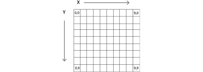
12.2 The Display Surface

The Display Surface (aka the display) is the most important part of a pygame game.

It is the main window display of your game and can be of any size, however you

can only have one Display Surface.

In many ways the Display Surface is like a blank piece of paper on which you

can draw. The surface itself is made up of pixels which are numbered from 0,0 in

the top left hand corner with the pixel locations being indexed in the x axis and the

y axis. This is shown below:

The above diagram illustrates how pixels within a Surface are indexed. Indeed a

Surface can be used to draw lines, shapes (such as rectangles, squares, circles and

elipses), display images, manipulate individual pixel s etc. Lines are drawn from one

pixel location to another (for example from location 0,0 to location 9,0 which

would draw a line across the top of the above display surface). Images can be

displayed within the display surface given a starting point such as 1, 1.

The Display Surface is created by the pygame.display.set_mode()

function. This function takes a tuple that can be used to specify the size of the

Display Surface to be returned. For example:

display_surface = pygame.display.set_mode((

400, 300))

This will create a Display Surface (window) of 400 by 300 pixels.

Once you have the Display Surface you can ﬁll it with an appropriate back-

ground colour (the default is black) however if you want a different background

colour or want to clear everything that has previously been drawn on the surface,

then you can use the surface’s ﬁll() method:

WHITE = (255, 255, 255)

display_surface.fill(WHITE)

The ﬁll method takes a tuple that is used to deﬁne a colour in terms of Red,

Green and Blue (or RGB) colours. Although the above examples uses a meaningful

name for the tuple representing the RGB values used for white; there is of course no

requirement to do this (although it is considered good practice).

126 12 Building Games with pygame

To aid in performance any changes you make to the Display Surface actually

happen in the background and will not be rendered onto the actual display that the

user sees until you call the update() or ﬂip() methods on the surface. For

example:

• pygame.display.update()

• pygame.display.flip()

The update() method will redraw the display with all changes made to the

display in the background. It has an optional parameter that allows you to specify

just a region of the display to update (this is deﬁned using a Rect which represents

a rectangular area on the screen). The ﬂip() method always refreshes the whole of

the display (and as such does exactly the same as the update() method with no

parameters).

Another method, which is not speciﬁcally a Display Surface method, but which

is often used when the display surface is created, provides a caption or title for the

top level window. This is the pygame.display.set_caption() function.

For example:

pygame.display.set

caption('Hello World')

This will give the top level window the caption (or title) ‘Hello World’.

12.3 Events

Just as the Graphical User Interface systems described in earlier chapters have an

event loop that allows the programmer to work out what the user is doing (in those

cases this is typically selecting a menu item, clicking a button or entering data etc.);

pygame has an event loop that allows the game to work out what the player is

doing. For example, the user may press the left or right arrow key. This is repre-

sented by an event.

12.3.1 Event Types

Each event that occurs has associated information such as the type of that event. For

example:

• Pressing a key will result in a KEYDOWN type of event, while releasing a key

will result in a KEYUP event type.

• Selecting the window close button will generate a QUIT event type etc.

• Using the mouse can generate MOUSEMOTION events as wel l as

MOUSEBUTTOND OWN and MOUSEBUTTONUP event types.

12.2 The Display Surface 127

• Using a Joystick can generate several different types of event including

JOYAXISMOTIO N, JOYBA LLMOTION, JOYBUTTONDOWN and JOYBU

TTONUP.

These event types tell you what occurred to generate the event. This means that

you can choose which types of events you want to deal with and ignore other

events.

12.3.2 Event Information

Each type of event object provides information associated with that event. For

example a Key oriented event object will provide the actual key pressed while a

mouse oriented event object will provide information on the position of the mouse,

which button was pressed etc. If you try an access an attribute on an event that does

not support that attribute, then an error will be generated.

The following lists some of the attributes available for different event types:

• KEYDOWN and KEYUP, the event has a key attribute and a mod attribute

(indicating if any other modifying keys such as Shift are also being pressed).

• MOUSEBUTTONU P and MOUSEBUTTONDOWN has an attribute pos that holds a

tuple indicating the mouse location in terms of x and y coordinates on the

underlying surface. It also has a button attribute indicating which mouse was

pressed.

• MOUSEMOTION has pos, rel and buttons attributes. The pos is a tuple indi-

cating the x and y location of mouse cursor. The real attribute indicates the

amount of mouse movement and buttons indicates the state of the mouse

buttons.

As an example if we want to check for a keyboard event type and then check that

the key pressed was the space bar, then we can write:

if event.type == pygame.KEYDOWN:

# Check to see which key is presse

if event.key == pygame.K_SPACE:

print('space')

This indicates that if it is a key pressed event and that the actual key was the

space bar; then print the string ‘space’.

There are many keyboard constants that are used to represent the keys on the

keyboard and pygame.K_SPACE constant used above is just one of them.

All the keyboard constants are preﬁxed with ‘K_’ followed by the key or the

name of the key, for example:

128 12 Building Games with pygame

• K_TAB, K_SPACE, K_PLUS, K_0, K_1, K_AT, K_a, K_b, K_z, K_DELTE,

K_DOWN, K_LEFT, K_RIGHT, K_LE FT etc.

Further keyboard constants are provided for modiﬁer states that can be combined

with the above such as KMOD_SHIFT, KMOD_CAPS, KMOD_CTRL and

KMOD_ALT.

12.3.3 The Event Queue

Events are supplied to a pygame application via the Event Queue.

The Event Queue is used to co llect together events as they happen. For ex ample,

let us assume that a user clicks on the mouse twice and a key twice before a

program has a chance to process them; then there will be four events in the Event

Queue as shown below:

The application can then obtain an iterable from the event queue and process

through the events in turn. While the program is processing these events further

events may occur and will be added to the Event Queue. When the program has

ﬁnished processing the initial collection of events it can obtain the next set of events

to process.

One signiﬁcant advantage of this approach is that no events are ever lost; that is

if the user clicks the mouse twice while the program is processing a previous set of

events; they will be recorded and added to the event queue. Another advantage is

that the events will be presented to the program in the order that they occurred.

The pygame.event.get() function will read all the events currently on the

Event Queue (removing them from the event queue). The method returns an

EventList which is an iterable list of the events read. Each event can then be

processed in turn. For example:

for event in pygame.event.get():

if event.type == pygame.QUIT:

print('Received Quit Event:')

elif event.type == pygame.MOUSEBUTTONDOWN:

print('Received Mouse Event')

elif event.type == pygame.KEYDOWN:

print('Received KeyDown Event')

12.3 Events 129

In the above code snippet an EventList is obtained from the Event Queue

containing the current set of events. The for loop then processes each event in turn

checking the type and printing an appropriate message.

You can use this approach to trigger appropriate behaviour such as moving an

image around the screen or calculating the players score etc. However, be aware

that if this behaviour takes too long it can make the game difﬁcult to play (although

the examples in this chapter and the next are simple enough that this is not a

problem).

12.4 A First pygame Application

We are now at the point where we can put together what we have looked at so far

and create a simple pygame application.

It is common to create a hello world style program when using a new pro-

gramming language or using a new application framework etc. The intention is that

the core elements of the language or framework are explored in order to generate

the most basic form of an application using the language or framework. We will

therefore implement the most basic application possible using pygame.

The application we will create will display a pygame window, with a ‘Hello

World’ title. We will then be able to quit the game. Although technically speaking

this isn’t a game, it does possess the basic architecture of a pygame application.

The simple HelloWorld game will initialise pygame and the graphical dis-

play. It wi ll then have a main game playing loop that will continue until the user

selects to quit the application. It will then shut down pygame. The display created

by the program is shown below for both Mac and Windows operating systems:

To quit the program click on the exit button for the windowing system you are

using.

130 12 Building Games with pygame

The simple HelloWorld game is given below:

import pygame

def main():

print('Starting Game')

print('Initialising pygame')

pygame.init()

# Required by every pygame applicatio

print('Initialising HelloWorldGame')

pygame.display.set_mode((200, 100))

pygame.display.set_caption('Hello World')

print('Update display')

pygame.display.update()

print('Starting main Game Playing Loop')

running = True

while running:

for event in pygame.event.get():

if event.type == pygame.QUIT:

print('Received Quit Event:', event)

running = False

print('Game Over')

pygame.quit()

if __name__ == '__main__':

main()

There are several key steps highlighted by this example, these steps are:

1. Import pygame. pygam e is of course not one of the default modules available

within Python. You must ﬁrst import pygame into you code. The import

pygame statement imports the pygame module into your code and makes the

functions and classes in pygame available to you (note the capitalisation -

pygame is not the same module name as PyGame). It is also common to ﬁnd

that programs import

• from pygame.locals import *

• This adds several constants and functions into the namespace of your pro-

gram. In this very simple example we have not needed to do this.

2. Initialise pygame. Almos t every pygame module needs to be initialised in some

way and the simplest way to do this is to call pygame.init() . This will do

what is required to set the pygame environment up for use. If you forget to call

this funct ion you will typically get an error message such as pygame.error:

video system not initialised (or something similar). If you get such a

12.4 A First pygame Application 131

method check to see that you have called pygame.init(). Note that you can

initialise individual pygame modules (for example the pygame.font module

can be initialised using pygame.font.init()) if required. However

pygame.init( ) is the most commonly used approach to setting up pygame.

3. Set up the display. Once you have initialised the pygame framework you can

setup the display. In the above code example, the display is set up using the

pygame.displ ay.set_mode() function. This function takes a tuple

specifying the size of the window to be created (in this case 200 pixels wide by

100 pixels high). Note that if you try and invoke this function by passing in two

parameters instead of a tuple, then you will get an error. This function returns

the drawing surface or screen/window that can be used to display items within

the game such as icons, messages, shapes etc. As our example is so simple we

do not bother saving it into a variable. However, anything more complex than

this will need to do so. We also set the window/frame’s caption (or title). This is

displayed in the title bar of the window.

4. Render the display. We now call the pygame.display.update() func-

tion. This function causes the current details of the display to be drawn. At the

moment this is a blank window. However, it is common in games to perform a

series of updates to the display in the background and then when the program is

ready to update the display to call this function. This batches a series of update s

and the causes the display to be refreshed. In a complex display it is possible to

indicate which parts of the display need to be redrawn rather than redrawing the

whole window. This is done by passing a parameter into the update()

function to indicate the rectangle to be redrawn. However, our example is so

simple we are ok with redrawing the whole window and therefore we do not

need to pass any parameters to the function.

5. Main game playing loop. It is common to have a main game playing loop that

drives the processing of user inputs, modiﬁes the state of the game and updates

the display. This is represented above by the while running: loop. The local

variable running is initialised to True. This means that the while loop

ensures that the game continues until the user selects to quit the game at which

point the running variable is set to False which causes the loop to exit. In

many cases this loop will call update() to refresh the display. The above

example does not do this as nothi ng is changed in the display. However the

example developed later in this chapter will illustrate this idea.

6. Monitor for events that drive the game. As mentioned earlier the event queue

is used to allow user inputs to be queued and then processed by the game. In the

simple example shown above this is represented by a for loop that receives

events using pygame.event. get() and then checking to see if the event is

a pygame.QUIT event. If it is, then it sets the running ﬂag to False. Which

will cause the main while loop of the game to terminate.

7. Quit pygame once ﬁnished. In pygame any module that has an init()

function also has an equivalent quit() function that can be used to perform

any cleanup operations. As we called init() on the pygame module at the

132 12 Building Games with pygame

start of our program we wi ll therefore need to call pygame.quit() at the end

of the program to ensure everything is tidied up appropriately.

The output generated from a sample run of this program is given below:

pygame 1.9.6

Hello from the pygame community.

https://www.pygame.org/contribute.html

Starting Game

Initialising pygame

Initialising HelloWorldGame

Update display

Starting main Game Playing Loop

Received Quit Event: <Event(12-Quit {})>

Game Over

12.5 Further Concepts

There are very many facilities in pygame that go b eyond what we can cover in this

book, however a few of the more common are discussed below.

Surfaces are a hierarchy. The top level Display Surface may contain other

surfaces that may be used to draw images or text. In turn containers such as Panels

may render surfaces to display images or text etc.

Other types of surface. The primary Display Surface is not the only surfa ce in

pygame. For example, when an image, such as a PNG or JPEG image is loaded into

a game then it is rendered onto a surface. This surface can then be displayed within

another surface such as the Display Surface. This means that anything you can do to

the Display Surface you can do with any other surface such as draw on it, put text

on it, colour it, add another icon onto the surface etc.

Fonts. The pygame.font.Font object is used to create a Font that can be

used to render text onto a surface. The render method returns a surface with the text

rendered on it that can be displayed within another surface such as the Display

Surface. Note that you cannot write text onto an existing surface you must always

obtain a new surface (using render) and then add that to an existing surface. The

text can only be displayed in a single line and the surface holding the text will be of

the dimensions required to render the text. For example:

text_font = pygame.font.Font('freesansbold.ttf', 18)

text_surface = text_font.render('Hello World', antialias=True,

color=BLUE)

This creates a new Font object using the speciﬁed font with the speciﬁed font

size (in this case 18). It will then render the string ‘Hello World’ on to a new surface

using the speciﬁed font and font size in Blue. Specif ying that antialias is True

indicates that we would like to smooth the edges of the text on the screen.

12.4 A First pygame Application 133

Rectangles (or Rects). The pygame.Rect class is an object used to represent

rectangular coordi nates. A Rect can be created from a combination of the top left

corner coordinates plus a width and height. For ﬂexibility many functions that

expect a Rect object can also be given a Rectlike list; this is a list that contains the

data necessary to create a Rect object. Rects are very useful in a pygame Game as

they can be used to deﬁne the borders of a game object. This means that they can be

used within games to detect if two objects have collided. This is made particularly

easy because the Rect class provides several collision detection methods:

The class also provides several other utility methods such as move() which

moves the rectangle and inﬂate() which can grow or shrink the rectangles size.

Drawing shapes. The pygame.draw module has numerous functions that can

be used to draw lines and shapes onto a surface, for example:

pygame.draw.rect(display_surface, BLUE, [x, y, WIDTH, HEIGHT])

This will draw a ﬁlled blue rectangle (the default) onto the display surface. The

rectangle will be located at the location indicated by x and y (on the surface). This

indicates the top left hand corner of the rectangle. The width and height of the

rectangle indicate its size. Note that these dimensions are deﬁned within a list which

is a structure referred to as being rect like (see below). If you do not want a ﬁlled

rectangle (i.e. You just want the outline) then you can use the optional width

parameter to indicate the thickness of the outer edge. Other methods available

include:

• pygame.draw. polygon() draw a shape with any number of sides

• pygame.draw. circle() draw a circle around a point

• pygame.draw. ellipse() draw a round shape inside a rectangle

• pygame.draw. arc() draw a partial section of an ellipse

• pygame.draw. line() draw a straight line segment

• pygame.draw. lines() draw multiple contiguous line segments

• pygame.draw. aaline() draw ﬁne antialiased lines

• pygame.draw. aalines() draw a connected sequence of antialiased lines

• pygame.Rect.contains() test if one rectangle is inside another

• pygame.Rect.collidepoint() test if a point is inside a rectangle

• pygame.Rect.colliderect() test if two rectangles overlap

• pygame.Rect.collidelist() test if one rectangle in a list intersects

• pygame.Rect.collidelistall() test if all rectangles in a list intersect

• pygame.Rect.collidedict() test if one rectangle in a dictionary intersects

• pygame.Rect.collidedictall() test if all rectangles in a dictionary intersect

134 12 Building Games with pygame

Images. The pygame.image module contains functions for loading, saving

and transforming images. When an image is loaded into pygame, it is represented

by a Surface object. This means that it is possible to draw, manipulate and process

an image in exactly the same way as any other surface which provides a great deal

of ﬂexibility.

At a min imum the module only supports loading uncompressed BMP images but

usually also supports JPEG, PNG, GIF (non-animated), BMP, TIFF as well as other

formats. However, it only supports a limited set of formats when saving images;

these are BMP, TGA, PNG and JPEG.

An image can be loaded from a ﬁle using:

image_surface = pygame.image.load(filename).convert()

This will load the image from the speciﬁed ﬁle onto a surface.

One thing you might wonder at is the use of the conve rt() method on the

object returned from the pygame.image.load() function. This function

returns a Surface that is used to display the image contained in the ﬁle. We call the

method convert() on this Surface, not to convert the image from a particular

ﬁle format (such as PNG, or JPEG) instead this method is used to convert the pixel

format used by the Surface. If the pixel format used by the Surface is not the

same as the display format, then it will need to be converted on the ﬂy each time the

image is displayed on the screen ; this can be a fairly time consuming (and

unnecessary) proces s. We therefore do this once when the image is loaded which

means that it should not hinder runtime performance and may improve performance

signiﬁcantly on some systems.

Once you have a surface containing an image it can be render ed onto another

surface, such as the display surface using the Surface.blit() method. For

example:

display_surface.blit(image_surface, (x, y))

Note that the position argument is a tuple specifying the x and y coordinates to

the image on the display surface.

Strictly speaking the blit() method draws one surface (the source surface)

onto another surface at the destination coordinates. Thus the target surface does not

beed to be the top level display surface.

Clock.AClock object is an object that can be used to track time. In particular

it can be used to deﬁne the frame rate for the game. That is the number of frames

rendered per second. This is done using the Clock.tick() method. This method

should be called once (and only once) per frame. If you pass the optional

framerate argument to the tick() the function, then pygame will ensure that

12.5 Further Concepts 135

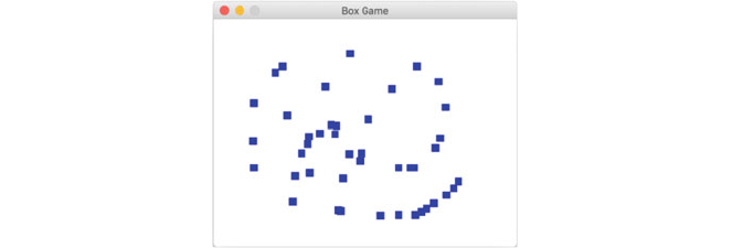
the games refresh rate is slower then the the given ticks per second. This can be

used to help limit the runtime speed of a game. By calling clock.tick

(30) once per frame, the program will never run at more than 30 frames per

second.

12.6 A More Interactive pygame Application

The ﬁrst pygame application we looked at earlier just displayed a window with the

caption ‘Hello World’. We can now extend this a little by playing with some of the

features we have looked at above.

The new application will add some mouse event handling. This will allow us to

pick up the location of the mouse when the user clicked on the window and draw a

small blue box at that point.

If the user clicks the mouse multiple times we will get multiple blue boxes being

drawn. This is shown below.

This is still not much of a game but does make the pygame application more

interactive.

The program used to generate this application is presented below:

import pygame

FRAME_REFRESH_RATE = 30

BLUE = (0, 0, 255)

BACKGROUND = (255, 255, 255) # White

WIDTH = 10

HEIGHT = 10

def main():

print('Initialising PyGame')

pygame.init()

# Required by every PyGame applicatio

136 12 Building Games with pygame

print('Initialising Box Game')

display_surface = pygame.display.set_mode((400, 300))

pygame.display.set_caption('Box Game')

print('Update display')

pygame.display.update()

print('Setup the Clock')

clock = pygame.time.Clock()

# Clear the screen of current contents

display_surface.fill(BACKGROUND)

print('Starting main Game Playing Loop')

running = True

while running:

for event in pygame.event.get():

if event.type == pygame.QUIT:

print('Received Quit Event:', event)

running = False

elif event.type == pygame.MOUSEBUTTONDOWN:

print('Received Mouse Event', event)

x, y = event.pos

pygame.draw.rect(display_surface, BLUE, [x, y,

WIDTH, HEIGHT])

# Update the display

pygame.display.update()

# Defines the frame rate - the number of frames per

second

# Should be called once per frame (but only once)

clock.tick(FRAME_REFRESH_RATE)

print('Game Over')

# Now tidy up and quit Python

pygame.quit()

if __name__ == '__main__':

main()

Note that we now need to record the display surface in a local variable so that we

can use it to draw the blue rectangles. We also need to call the pygame.dis-

play.update() function each time round the main while loop so that the new

rectangles we have drawn as part of the event processing for loop are displayed to

the user.

We also set the frame rate each time round the main while loop. This should

happen once per frame (but only once) and uses the clock object initialised at the

start of the program.

12.6 A More Interactive pygame Application 137

12.7 Alternative Approach to Processing Input Devices

There are actually two ways in which inputs from a device such as a mouse,

joystick or the keyboard can be processed. One approach is the Event based model

described earlier. The other approach is the State based approach.

Although the Event based approach has many advant ages is has two

disadvantages:

• Each event represents a single action and continuous actions are not explicitly

represented. Thus if the user presses both the X key and the Z key then this will

generate two events and it will be up to the program to determine that they have

been pressed at the same time.

• It is also up to the program to determine that the user is still pressing a key (by

noting that no KEYUP event has occurred).

• Both of these are possible but can be error prone.

An alternative approach is to use the State based approach. In the state based

approach the program can directly check the state of a input device (such as a key or

mouse or keyboard). For example, you can use pygame.key.g et_pressed()

which returns the state of all the keys. This can be used to determine if a speciﬁc

key is being pressed at this moment in time. For example, pygame.key.

get_pressed()[pygame.K_SPACE] can be used to check to see if the space

bar is being pressed.

This can be used to determine what action to take. If you keep checking that the

key is pressed then you can keep performing the associated action. This can be very

useful for continues actions in a game such as moving an object etc.

However, if the user presses a key and then releases it before the program checks

the state of the keyboard then that input will be missed.

12.8 pygame Modules

There are numerous modules provided as part of pygame as well as associated

libraries. Some of the core modules are listed below:

• pygame.displ ay This module is used to control the display window or

screen. It provides facilities to initialise and shutdown the display module. It can

be used to initialise a window or screen. It can also be used to cause a window

or screen to refresh etc.

138 12 Building Games with pygame

•

pygame.event This module manages events and the event queue. For example

pygame.event.get() retrieves events from the event queue,

pygame.event.poll() gets a single event from the queue and

pygame.event.peek() tests to see if there are any event types on the queue.

• pygame.draw The draw module is used to draw simple shapes onto a

Surface. For example, it provides functions for drawing a rectangle

(pygame.draw.rect), a polygon, a circle, an ellipse, a line etc.

• pygame.font The font module is used to create and render TrueType fonts

into a new Surface object. Most of the features associated with fonts are sup-

ported by the pygame.font.Font class. Free standing module functions

allow the module to be initialised and shutdown, plus functions to access fonts

such as pygame.font.get_fonts() which provides a list of the currently

available fonts.

• pygame.image This module allows images to be saved and loaded. Note that

images are loaded into a Surface object (there is no Image class unlike many

other GUI oriented frameworks).

• pygame.joystick The joystick module provides the Joystick object and

several supporting functions. These can be used for interacting with joysticks,

gamepads and trackballs.

• pygame.key This module provides support for working with inputs from the

keyboard. This allows the input keys to be obtained and modiﬁer keys (such as

Control and Shift) to be identiﬁed. It also allows the approach to repeating keys

to be speciﬁed.

• pygame.mouse This module provides facilities for working with mouse input

such as obtaining the current mouse position, the state of mouse buttons as well

as the image to use for the mouse.

• pygame.time This is the pygame module for managing timing within a game.

It provides the pygame.time.Clock class that can be used to track time.

12.9 Online Resources

There is a great deal of information available on pygame including:

•

https://www.pygame.org The pygame home page.

•

http://www.libsdl.org/ SDL (Simple Directmedia Layer) documentation.

• news://gmane.comp.python.pygame The ofﬁcial pygame news group.

12.8 pygame Modules 139

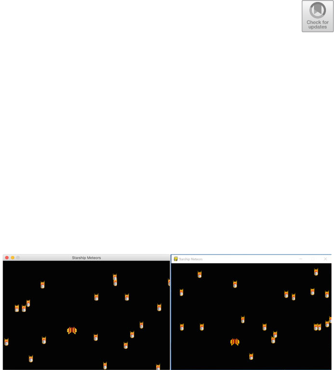
Chapter 13

StarshipMeteors pygame

13.1 Creating a Spaceship Game

In this chapter we will create a game in which you pilot a starship through a ﬁeld of

meteors. The longer you play the game the larger the number of meteors you will

encounter. A typical display from the game is shown below for a Apple Mac and a

Windows PC:

We will implement several classes to represent the entities within the game.

Using classes is not a required way to implement a game and it should be noted that

many developers avoid the use of classes. However, using a class allows data

associated with an object within the game to be maintained in one place; it also

simpliﬁes the creation of multiple instances of the same object (such as the meteors)

within the game.

J. Hunt, Advanced Guide to Python 3 Programming,

Undergraduate Topics in Computer Science,

https://doi.org/10.1007/978-3-030-25943-3_13

141

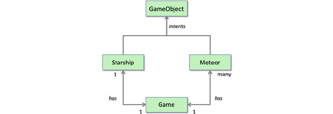
The classes and their relationships are shown below:

This diagram shows that the Starship and Meteor classes will extend a class

called GameObject.

In turn it also shows that the Game has a 1:1 relationship with the Starship class.

That is the Game holds a reference to one Starship and in turn the starship holds a

single reference back to the Game.

In contrast the Game has a 1 to many relationship with the Meteor class. That

is the Game object holds references to many Meteors and each Meteor holds a

reference back to the single Game object.

13.2 The Main Game Class

The ﬁrst class we will look at will be the Game class itself.

The Game class will hold the list of meteors and the starship as well as the main

game playing loop.

It will also initialise the main window display (for example by setting the size

and the caption of the window).

In this case we will store the display surface returned by the pygame.dis-

play.set_mode() function in an attribute of the Game object called dis-

play_surface. This is because we will need to use it later on to display the

starship and the meteors.

We will also hold onto an instance of the pygame.time.C lock() class that

we will use to set the fram e rate each time round the main game playing while loop.

The basic framework of our game is shown below; this listing provides the basic

Game class and the main method that will launch the game. The game also deﬁnes

three global constants that will be used to deﬁne the frame refresh rate and the size

of the display.

142 13 StarshipMeteors pygame

import pygame

# Set up Global 'constants'

FRAME_REFRESH_RATE = 30

DISPLAY_WIDTH = 600

DISPLAY_HEIGHT = 400

class Game:

""" Represents the game itself and game playing

loop """

def __init__(self):

print('Initialising PyGame')

pygame.init()

# Set up the display

self.display_surface =

pygame.display.set_mode((DISPLAY_WIDTH, DISPLAY_HEIGHT))

pygame.display.set_caption('Starship Meteors')

# Used for timing within the program.

self.clock = pygame.time.Clock()

def play(self):

is_running = True

# Main game playing Loop

while is_running:

# Work out what the user wants to do

for event in pygame.event.get():

if event.type == pygame.QUIT:

is_running = False

elif event.type == pygame.KEYDOWN:

if event.key == pygame.K_q:

is_running = False

# Update the display

pygame.display.update()

# Defines the frame rate

self.clock.tick(FRAME_REFRESH_RATE)

# Let pygame shutdown gracefully

pygame.quit()

def main():

print('Starting Game')

game = Game()

game.play()

print('Game Over')

if __name__ == '__main__':

main()

13.2 The Main Game Class 143

The main play() method of the Game class has a loop that will continue until

the user selects to quit the game. They can do this in one of two ways, either by

pressing the ‘q’ key (represented by the event.key K_q) or by clicking on the

window close button. In either case these events are picked up in the main event

processing for loop within the main while loop method.

If the user does not want to quit the game then the display is updated (refreshed)

and then the clock.tick() (or frame) rate is set.

When the user selects to quit the game then the main while loop is terminated

(the is_running ﬂag is set to False) and the pygame.quit() method is

called to shut down pygame.

At the moment this not a very interactive game as it does not do anything except

allow the user to quit. In the next section we will add in behaviour that will allow us

to display the space ship within the display.

13.3 The GameObject Class

The GameObject class deﬁnes three methods:

The load_image() method can be used to load an image to be used to

visually represent the speciﬁc type of game object. The method then uses the width

and height of the image to deﬁne the width and height of the game object.

The rect() method returns a rectangle representi ng the current area used by

the game object on the underlying drawing surface. This differs from the images

own rect() which is not related to the location of the game object on the

underlying surface. Rects are very useful for comparing the location of one object

with another (for example when determining if a collision has occurred).

The draw() method draws the GameObjects’ image onto the display_-

surface held by the game using the GameObjects current x and y coordinates. It

can be overridden by subclasses if they wish to be drawn in a different way.

The code for the GameObject class is presented below:

class GameObject:

def load_image(self, filename):

self.image = pygame.image.load(filename).convert()

self.width = self.image.get_width()

self.height = self.image.get_height()

def rect(self):

""" Generates a rectangle representing the objects

location

and dimensions """

144 13 StarshipMeteors pygame

return pygame.Rect(self.x, self.y, self.width,

self.height)

def draw(self):

""" draw the game object at the

current x, y coordinates """

self.game.display_surface.blit(self.image, (self.x,

self.y))

The GameO bject class is directly extended by the Starship class and the

Meteor class.

Currently there are only two types of game elements, the starship and the

meteors; but this could be extended in future to planets, comets, shooting stars etc.

13.4 Displaying the Starship

The human p layer of this game wi ll control a starship that can be moved around the

display.

The Starship will be represented by an instance of the class Starship. This

class will extend the GameObject class that holds common behaviours for any

type of element that is represented within the game.

The Starship class deﬁnes its own __init__() method that takes a reference

to the game that the starship is part of. This initialisation method sets the initial

starting location of the Starship as half the width of the display for the x coordinate

and the display height minus 40 for the y coordinate (this gives a bit of a buffer

before the end of the screen). It then uses the load_image() method from the

GameObject parent class to load the image to be used to represent the

Starship. This is held in a ﬁle called starship.png. For the moment we will

leave the Starship class as it is (how ever we will return to this class so that we

can make it into a movable object in the next section).

The current version of the Starship class is given below:

class Starship(GameObject):

""" Represents a starship"""

def __init__(self, game):

self.game = game

self.x = DISPLAY_WIDTH / 2

self.y = DISPLAY_HEIGHT - 40

self.load

image('starship.png')

13.3 The GameObject Class 145

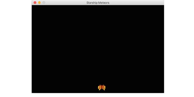
In the Game class we will now add a line to the __init__() method to

initialise the Starship object. This line is:

# Set up the starship

self.starship = Starship(self)

We will also add a line to the main while loop within the play() method just

before we refresh the display. This line will call the draw() method on the starship

object:

# Draw the starship

self.starship.draw()

This will have the effect of drawing the starship onto the windows drawing

surface in the background before the display is refreshed.

When we now run this version of the StarshipMeteor game we now see the

Starship in the display:

Of course at the moment the starship does not move; but we will address that in

the next section.

13.5 Moving the Spaceship

We want to be able to move the Starship about within the bounds of the display

screen.

To do this we need to change the starships x and y coordinates in response to the

user pressing various keys.

We will use the arrow keys to move up and down the screen or to the left or right

of the screen. To do this we will deﬁne four methods within the Stars hip class;

these methods will move the starship up, down, left and right etc.

146 13 StarshipMeteors pygame

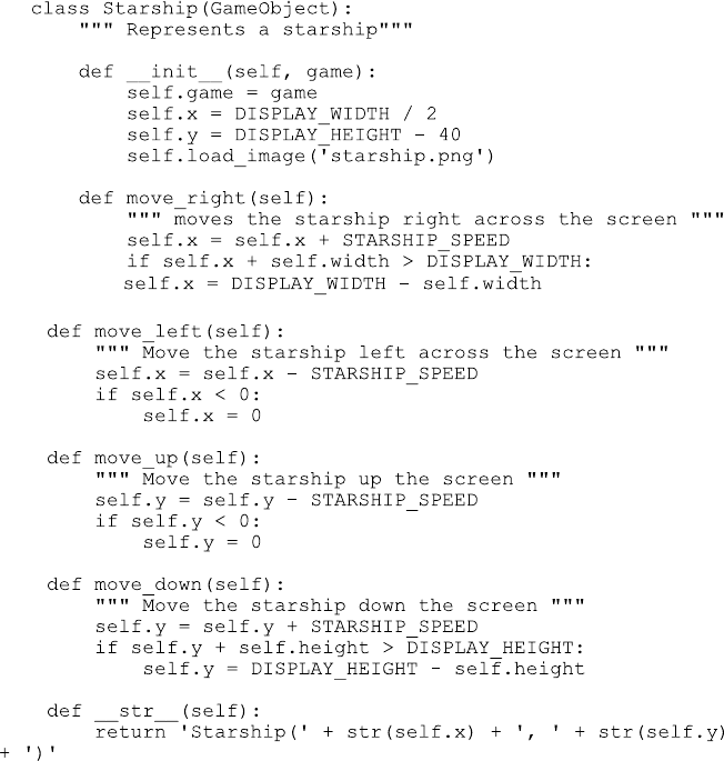
The updated Starship class is shown below:

This version of the Starship class deﬁnes the various move methods. These

methods use a new global value STARSHIP_SPEED to determine how far and

how fast the Starship moves. If you want to change the speed that the Starship

moves then you can change this global value.

Depending upon the direction intended we will need to modify either the x or y

coordinate of the Starship.

• If the starship moves to the left then the x coordinate is reduced by

STARSHIP_SPE ED,

• if it moves to the right then the x coordinate is increased by

STARSHIP_SPE ED,

• in turn if the Starship moves up the screen then the y coordinate is decremented

by STARSHIP_SPEED,

13.5 Moving the Spaceship 147

• but if it moves down the screen then the y coordinate is increased by

STARSHIP_SPE ED.

Of course we do not want our Starship to ﬂy off the edge of the screen and so a

test must be made to see if it has reached the boundaries of the screen. Thus tests are

made to see if the x or y values have gone below Zero or above the

DISPLAY_WIDTH or DISPLAY_HEIGHT values. If any of these conditions are

met then the x or y values are reset to an appropriate default.

We can now use these methods with player input. This player input will indicate

the direction that the player wants to move the Starship. As we are using the left,

right, up and down arrow keys for this we can extend the event processing loop that

we have already deﬁned for the main game playing loop. As with the letter q, the

event keys are preﬁxed by the letter K and an underbar, but this time the keys are

named K_LEFT, K_RIGHT, K_UP and K_DOWN.

When one of these keys is pressed then we will call the appropriate move

method on the starship object already held by the Game object.

The main event processing for loop is now:

# Work out what the user wants to do

for event in pygame.event.get():

if event.type == pygame.QUIT:

is_running = False

elif event.type == pygame.KEYDOWN:

# Check to see which key is pressed

if event.key == pygame.K_RIGHT:

# Right arrow key has been presse

# move the player right

self.starship.move_right()

elif event.key == pygame.K_LEFT:

# Left arrow has been pressed

# move the player left

self.starship.move_left()

elif event.key == pygame.K_UP:

self.starship.move_up()

elif event.key == pygame.K_DOWN:

self.starship.move_down()

elif event.key == pygame.K_q:

running = False

However, we are not quite ﬁnished. If we try and run this version of the program

we will get a trail of Starships drawn across the screen; for example:

148 13 StarshipMeteors pygame

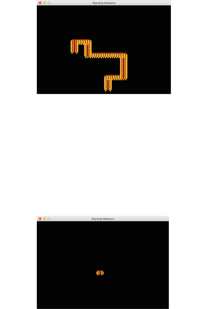
The problem is that we are redrawing the starship at a different position; but the

previous image is still present.

We now have two choices one is to mere ly ﬁll the whole screen with black;

effectively hiding anythi ng that has been drawn so far; or alternatively we could just

draw over the area used by the previous image position. Which approach is adopted

depends on the particular scenario represented by your game. As we will have a lot

of meteors on the screen once we have added them; the easiest option is to over-

write everything on the screen before redrawing the starship. We will therefore add

the following line:

# Clear the screen of current contents

self.display_surface.ﬁll(BACKGROUND)

This line is added just before we draw the Starship within the main game playing

while loop.

Now when we move the Starship the old image is removed before we draw the

new image:

One point to note is that we have also deﬁned another global value

BACKGROUND used to hold the background colour of the game playing surface.

This is set to black as shown below:

13.5 Moving the Spaceship 149

#Deﬁne default RGB colours

BACKGROUND = (0, 0, 0)

If you want to use a different background colour then change this global value.

13.6 Adding a Meteor Class

The Meteor class will also be a subclass of the GameObject class. However, it

will only provide a move_down() method rather than the variety of move

methods of the Starship.

It will also need to have a random starting x coordinate so that when a meteor is

added to the game its starting position will vary. This random position can be

generated using the random.randint() function using a value between 0 and

the width of the drawing surface. The meteor will also start at the top of the screen

so will have a different initial y coordinate to the Starship. Finally, we also want our

meteors to have different speeds; this can be another random number between 1 and

some speciﬁed maximum meteor speed.

To support these we need to add random to the modules being imported and

deﬁne several new global values, for example:

import pygame, random

INITIAL_METEOR_Y_LOCATION = 10

MAX_METEOR_SPEED = 5

We can now deﬁne the Meteor class:

class Meteor(GameObject):

""" represents a meteor in the game """

def __init__(self, game):

self.game = game

self.x = random.randint(0, DISPLAY_WIDTH)

self.y = INITIAL_METEOR_Y_LOCATION

self.speed = random.randint(1, MAX_METEOR_SPEED)

self.load_image('meteor.png')

def move_down(self):

""" Move the meteor down the screen """

self.y = self.y + self.speed

if self.y > DISPLAY_HEIGHT:

self.y = 5

def __str__(self):

return 'Meteor(' + str(self.x) + ', ' + str(self.y) +

')'

150 13 StarshipMeteors pygame

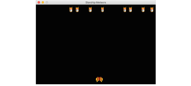
The __init__() method for the Meteor class has the same steps as the

Starship; the difference is that the x coordinate and the speed are randomly

generated. The image used for the Meteor is also different as it is ‘meteor.png’.

We have also implemented a move_down() method. This is essentially the

same as the Starships move_down().

Note that at this point we could create a subclass of GameObject called

MoveableGameObject (which extends GameObject) and push the move

operations up into that class and have the Meteor and Starship classes extend

that class. However we don’t really want to allow meteors to move just anywhere

on the screen.

We can now add the meteors to the Game class. We will add a new global value

to indicate the number of initial meteors in the game:

INITIAL

NUMBER

METEORS = 8

Next we will initialise a new attribute for the Game class that will hold a list of

Meteors. We will use a list here as we want to increase the number of meteors as the

game progresses.

To make this process easy we will use a list comprehension which allows a for

loop to run with the results of an expression captured by the list:

# Set up meteors

self.meteors = [Meteor(self) for _ in range(0,

INITIAL

NUMBER

METEORS)]

We now have a list of meteors that need to be displayed. We thus need to update

the while loop of the play() method to draw not only the starship but also all

the meteors:

# Draw the meteors and the starship

self.starship.draw()

for meteor in self.meteors:

meteor.draw()

The end result is that a set of meteor objects are created at random starting

locations across the top of the screen:

13.6 Adding a Meteor Class 151

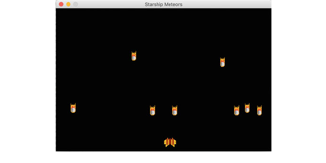
13.7 Moving the Meteors

We now want to be able to move the meteors down the screen so that the Starship

has some objects to avoid.

We can do this very easily as we have already implemented a move_down()

method in the Meteor class. We therefore only need to add a for loop to the main

game playing while loop that will move all the meteors. For example:

# Move the Meteors

for meteor in self.meteors:

meteor.move_down()

This can be added after the event processing for loop and before the screen is

refreshed/redrawn or updated.

Now when we run the game the meteors move and the player can navigate the

Starship between the falling meteors.

13.8 Identifying a Collision

At the moment the game will play for ever as there is no end state and no attempt to

identify if a Starship has collided with a meteor.

We can add Meteor/Starship collision detection using PyGame Rects. As

mentioned in the last chapter a Rect is a PyGame class used to represent rect-

angular coordinates. It is particularly useful as the pygame.Rect class provides

several collision detection methods that can be used to test if one rectangle (or

point) is inside another rectangle. We can therefore use one of the methods to test if

the rectangle around the Starship intersects with any of the rectangles around the

Meteors.

152 13 StarshipMeteors pygame

The GameObject class already provides a method rect() that will return a

Rect object representing the objects’ current rectangle with respect to the drawing

surface (esse ntially the box around the object representing its location on the

screen).

Thus we can write a collision detection method for the Game class using the

GameObject generated rects and the Rect class colliderect() method:

def _check_for_collision(self):

""" Checks to see if any of the meteors have collided with

the starship """

result = False

for meteor in self.meteors:

if self.starship.rect().colliderect(meteor.rect()):

result = True

break

return result

Note that we have followed the convention here of preceding the method name

with an underbar indicating that this method should be considered private to the

class. It should therefore never be called by anything outside of the Game class.

This convention is deﬁned in PEP 8 (Python Enhancement Proposal) but is not

enforced by the language.

We can now use this method in the main while loop of the game to check for a

collision:

# Check to see if a meteor has hit the shi

if self._check_for_collision():

starship_collided = True

This code snippet also introduces a new local variable starship_collided.

We will initially set this to False and is another condition under which the main

game playing while loop will terminate:

is_running = True

starship_collided = False

# Main game playing Loop

hile is

running and not starship

collided:

Thus the game playing loop will terminate if the user selects to quit or if the

starship collides with a meteor.

13.8 Identifying a Collision 153

13.9 Identifying a Win

We currently have a way to loose the game but we don ’t have a way to win the

game! However, we want the player to be able to win the game by surviving for a

speciﬁed period of time. We could represent this with a timer of some sort.

However, in our case we will represent it as a speciﬁc number of cycles of the main

game playing loop. If the player survives for this number of cycles then they have

won. For example:

# See if the player has won

if cycle_count == MAX_NUMBER_OF_CYCLES:

print('WINNER!')

break

In this case a message is printed out stating that the player won and then the

main game playing loop is terminated (using the break statement).

The MAX_NUMBER_OF_CYCLES global value can be set as appropriate, for

example:

MAX

NUMBER

CYCLES = 1000

13.10 Increasing the Number of Meteors

We could leave the game as it is at this point, as it is now possible to win or loose

the game. However, there are a few things that can be easily added that will enhance

the game playing experience. One of these is to increase the numbe r of Meteors on

the screen making it harder as the game progresses.

We can do this using a NEW_METEOR_CYCLE_INTERVAL.

NEW

METEOR

CYCLE

INTERVAL = 40

When this interval is reached we can add a new Meteor to the list of current

Meteors; it will then be automatically drawn by the Game class. For example:

# Determine if new meteors should be added

if cycle_count % NEW_METEOR_CYCLE_INTERVAL == 0:

self.meteors.append(Meteor(self))

154 13 StarshipMeteors pygame

Now every NEW_METEOR_CYCLE_INTERVAL another meteor will be added

at a random x coordinate to the game.

13.11 Pausing the Game

Another feature that many games have is the ability to pause the game. This can be

easily added by monitoring for a pause key (this could be the letter p represented by

the event_key pygame.K_p). When this is pressed the game could be paused until

the key is pressed again.

The pa use operation can be implemented as a method _pause() that will

consume all events until the appropriate key is pressed. For example:

def _pause(self):

paused = True

while paused:

for event in pygame.event.get():

if event.type == pygame.KEYDOWN:

if event.key == pygame.K_p:

paused =

False

break

In this method the outer while loop will loop until the paused local variable is

set too False. This only happens when the ‘p’ key is pressed. The break after the

statement setting paused to False ensures that the inner for loop is terminated

allowing the outer while loop to check the value of paused and terminate.

The _pause() method can be invoked during the game playing cycle by

monitoring for the ‘p’ key within the event for loop and calling the _pause()

method from there:

elif event.key == pygame.K_p:

self._pause()

Note that again we have indicated that we don’t expect the _pause() method

to be called from outside the game by preﬁxing the method name with an underbar

(‘_’).

13.10 Increasing the Number of Meteors 155

13.12 Displaying the Game Over Message

PyGame does not come with an easy way of creating a popup dialog box to display

messages such as ‘You Won’;or‘ You Lost’ which is why we have used print

statements so far. However, we could use a GUI framework such as wxPython to do

this or we could display a message on the display surface to indi cate whether the

player has won or lost.

We can display a mess age on the display surface using the pygame.font.

Font class. This can be used to create a Font object that can be rendered onto a

surface that can be displayed onto the main display surface.

We can therefore add a method _display_message() to the Game class

that can be used to display appropriate messages:

def _display_message(self, message):

""" Displays a message to the user on the screen """

print(message)

text_font = pygame.font.Font('freesansbold.ttf',48)

text_surface = text_font.render(message, True, BLUE, WHITE)

text_rectangle = text_surface.get_rect()

text_rectangle.center = (DISPLAY_WIDTH / 2,

DISPLAY_HEIGHT / 2)

self.display_surface.fill(WHITE)

self.display

surface.blit(text

surface, text

rectangle)

Again the leading underbar in the method name indicates that it should not be

called from outside the Game class.

We can now modify the main loop such that appropriate messages are displayed

to the user, for example:

# Check to see if a meteor has hit the ship

if self._check_for_collision():

starship_collided = True

self._display_message('Collision: Game Over')

156 13 StarshipMeteors pygame

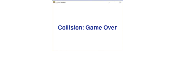
The result of the above code being run when a collision occurs is shown below:

13.13 The StarshipMeteors Game

The complete listing for the ﬁnal version of the StarshipMeteors game is given

below:

import pygame, random, time

FRAME_REFRESH_RATE = 30

DISPLAY_WIDTH = 600

DISPLAY_HEIGHT = 400

WHITE = (255, 255, 255)

BACKGROUND = (0, 0, 0)

INITIAL_METEOR_Y_LOCATION = 10

INITIAL_NUMBER_OF_METEORS = 8

MAX_METEOR_SPEED = 5

STARSHIP_SPEED = 10

MAX_NUMBER_OF_CYCLES = 1000

NEW

METEOR

CYCLE

INTERVAL = 40

13.12 Displaying the Game Over Message 157

class GameObject:

def load_image(self, filename):

self.image = pygame.image.load(filename).convert()

self.width = self.image.get_width()

self.height = self.image.get_height()

def rect(self):

""" Generates a rectangle representing the objects

location

and dimensions """

return pygame.Rect(self.x, self.y, self.width,

self.height)

def draw(self):

""" draw the game object at the

current x, y coordinates """

self.game.display_surface.blit(self.image, (self.x,

self.y))

class Starship(GameObject):

""" Represents a starship"""

def __init__(self, game):

self.game = game

self.x = DISPLAY_WIDTH / 2

self.y = DISPLAY_HEIGHT - 40

self.load_image('starship.png')

def move_right(self):

""" moves the starship right across the screen """

self.x = self.x + STARSHIP_SPEED

if self.x + self.width > DISPLAY_WIDTH:

self.x = DISPLAY_WIDTH - self.width

def move_left(self):

""" Move the starship left across the screen """

self.x = self.x - STARSHIP_SPEED

if self.x < 0:

self.x = 0

def move_up(self):

""" Move the starship up the screen """

self.y = self.y - STARSHIP_SPEED

if self.y < 0:

self.y = 0

def move_down(self):

""" Move the starship down the screen """

self.y = self.y + STARSHIP_SPEED

if self.y + self.height > DISPLAY

HEIGHT:

158 13 StarshipMeteors pygame

self.y = DISPLAY_HEIGHT - self.height

def __str__(self):

return 'Starship(' + str(self.x) + ', ' + str(self.y) +

')'

class Meteor(GameObject):

""" represents a meteor in the game """

def __init__(self, game):

self.game = game

self.x = random.randint(0, DISPLAY_WIDTH)

self.y = INITIAL_METEOR_Y_LOCATION

self.speed = random.randint(1, MAX_METEOR_SPEED)

self.load_image('meteor.png')

def move_down(self):

""" Move the meteor down the screen """

self.y = self.y + self.speed

if self.y > DISPLAY_HEIGHT:

self.y = 5

def __str__(self):

return 'Meteor(' + str(self.x) + ', ' + str(self.y) +

')'

class Game:

""" Represents the game itself, holds the main game playing

loop """

def __init__(self):

pygame.init()

# Set up the display

self.display_surface =

pygame.display.set_mode((DISPLAY_WIDTH, DISPLAY_HEIGHT))

pygame.display.set_caption('Starship Meteors')

# Used for timing within the program.

self.clock = pygame.time.Clock()

# Set up the starship

self.starship = Starship(self)

# Set up meteors

self.meteors = [Meteor(self) for _ in range(0,

INITIAL_NUMBER_OF_METEORS)]

def _check_for_collision(self):

""" Checks to see if any of the meteors have collided

ith the starship """

result = False

for meteor in self.meteors:

if self.starship.rect().colliderect(meteor.rect()):

result = True

13.13 The StarshipMeteors Game 159

break

return result

def _display_message(self, message):

""" Displays a message to the user on the screen """

text_font = pygame.font.Font('freesansbold.ttf',48)

text_surface = text_font.render(message, True, BLUE,

WHITE)

text_rectangle = text_surface.get_rect()

text_rectangle.center = (DISPLAY_WIDTH / 2,

DISPLAY_HEIGHT / 2)

self.display_surface.fill(WHITE)

self.display_surface.blit(text_surface, text_rectangle)

def _pause(self):

paused = True

while paused:

for event in pygame.event.get():

if event.type == pygame.KEYDOWN:

if event.key == pygame.K_p:

paused = False

break

def play(self):

is_running = True

starship_collided = False

cycle_count = 0

# Main game playing Loop

while is_running and not starship_collided:

# Indicates how many times the main game loop has

been run

cycle_count += 1

# See if the player has won

if cycle_count == MAX_NUMBER_OF_CYCLES:

self._display_message('WINNER!')

break

# Work out what the user wants to do

for event in pygame.event.get():

if event.type == pygame.QUIT:

is_running = False

elif event.type == pygame.KEYDOWN:

# Check to see which key is pressed

if event.key == pygame.K_RIGHT:

# Right arrow key has been pressed

# move the player right

self.starship.move_right()

elif event.key == pygame.K_LEFT:

# Left arrow has been pressed

160 13 StarshipMeteors pygame

# move the player left

self.starship.move_left()

elif event.key == pygame.K_UP:

self.starship.move_up()

elif event.key == pygame.K_DOWN:

self.starship.move_down()

elif event.key == pygame.K_p:

self._pause()

elif event.key == pygame.K_q:

is_running = False

# Move the Meteors

for meteor in self.meteors:

meteor.move_down()

# Clear the screen of current contents

self.display_surface.fill(BACKGROUND)

# Draw the meteors and the starship

self.starship.draw()

for meteor in self.meteors:

meteor.draw()

# Check to see if a meteor has hit the ship

if self._check_for_collision():

starship_collided = True

self._display_message('Collision: Game Over')

# Determine if new mateors should be added

if cycle_count % NEW_METEOR_CYCLE_INTERVAL == 0:

self.meteors.append(Meteor(self))

# Update the display

pygame.display.update()

# Defines the frame rate. The number is number of

frames per

# second. Should be called once per frame (but only

once)

self.clock.tick(FRAME_REFRESH_RATE)

time.sleep(1)

# Let pygame shutdown gracefully

pygame.quit()

def main():

print('Starting Game')

game = Game()

game.play()

print('Game Over')

if __name__ == '__main__':

main()

13.13 The StarshipMeteors Game 161

13.14 Online Resources

There is a great deal of information available on PyGame including:

•

https://www.pygame.org The PyGame home page.

•

https://www.pygame.org/docs/tut/PygameIntro.html PyGame tutorial.

•

https://www.python.org/dev/peps/pep-0008/ PEP8 Style Guide for Python

Code.

13.15 Exercises

Using the example presented in this chapter add the following:

• Provide a score counter. This could be based on the number of cycles the player

survives or the number of meteors that restart from the top of the screen etc.

• Add anothe r type of GameObject, this could be a shoot ing star that moves

across the screen horizontally; perhaps using an random starting y coordinate.

• Allow the game difﬁculty to be speci ﬁed at the start. This could affect the

number of initial met eors, the maximum speed of a meteor, the number of

shooting stars etc.

162 13 StarshipMeteors pygame

Part III

Testing

Chapter 14

Introduction to Testing

14.1 Introduction

This chapter considers the different types of tests that you might want to perform

with the systems you develop in Python. It also introduces Test Driven

Development.

14.2 Types of Testing

There are at least two ways of thinking about testing:

1. It is the process of executing a program with the intent of ﬁnding errors/bugs

(see Glenford Myers, The Art of Software Testing).

2. It is a process used to establish that software components fulﬁl the requirements

identiﬁed for them, that is that they do what they are supposed to do.

These two aspects of testing tend to have been emphasised at different points in the

software lifecycle. Error Testing is an intrinsic part of the development process, and

an increasing emphasis is being placed on making testing a central part of software

development (see Test Driven Development).

It should be noted that it is extremely difﬁcult—and in many cases impossible—

to prove that software works and is completely error free. The fact that a set of tests

ﬁnds no defects does not prove that the software is error-free. ‘Absence of evidence

is not evidence of absence!’. This was discussed in the late 1960s and early 1970s

by Dijkstra and can be summarised as:

Testing shows the presence, not the absence of bugs

Testing to establish that software components fulﬁl their contract involves

checking operations against their requi rements. Although this does happen at

J. Hunt, Advanced Guide to Python 3 Programming,

Undergraduate Topics in Computer Science,

https://doi.org/10.1007/978-3-030-25943-3_14

165

development time, it forms a major part of Quality Assurance (QA) and User

Acceptance testing. It should be noted that wi th the advent of Test-Driven

Development, the emphasis on testing against requirements during development has

become signiﬁcantly higher.

There are of course many other aspects to testing, for example, Performance

Testing which identiﬁes how a system will perform as various factors that affect that

system change. For example, as the number of concurrent requests increase, as the

number of processors used by the underlying hardware changes, as the size of the

database grows etc.

However you view testing, the more testing applied to a system the higher the

level of conﬁdence that the system will work as required.

14.3 What Should Be Tested?

An interesting question is ‘What aspects of your software system should be subject

to testing?’.

In general, anything that is repeatable should be subject to formal (and ideally

automated) testing. This includes (but is not limited to):

• The build process for all technologies involved.

• The deployment process to all platforms under consideration.

• The installation process for all runtime environments.

• The upgrade process for all supported versions (if appropriate ).

• The performance of the system/servers as loads increase.

• The stability for systems that must run for any period of time (e.g. 24  7

systems).

• The backup processes.

• The security of the system.

• The recovery ability of the system on failure.

• The functionality of the system.

• The integrity of the system.

Notice that only the last two of the above list might be what is commonly con-

sidered areas that would be subject to testing. However, to ensure the quality of the

system under consideration, all of the above are relevant. In fact, testing should

cover all aspects of the software development lifecycle and not just the QA phase.

During requirements gathering testing is the process of looking for missing or

ambiguous requirements. During this phase consideration should also be made with

regard to how the overall requirements will be tested, in the ﬁnal software system.

166 14 Introduction to Testing

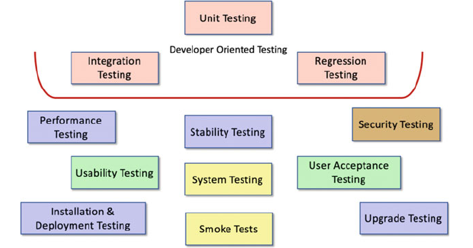
Test planning should also look at all aspects of the software under test for func-

tionality, usability, legal compliance, conformance to regul atory constraints, secu-

rity, performance, availability, resilience, etc. Testing should be driven by the need

to identify and reduce risk.

14.4 Testing Software Systems

As indi cated above there are a number of different types of testing that are

commonly used within industry. These types are:

• Unit Testing, which is used to verify the behaviour of individual components.

• Integration Testing that tests that when individual components are combined

together to provide higher-level functional units, that the combination of the

units operates appropriately.

• Regression Testing. When new components are added to a system, or existing

components are changed, it is necessary to verify that the new functionality does

not break any existing functionality. Such testing is known as Regression

Testing.

• Performance Testing is used to ensure that the systems’ performance is as

required and, within the design parameters, and is able to scale as utilisation

increases.

• Stability Testing represents a style of testing which attempts to simulate system

operation over an extended period of time. For example, for a online shopping

application that is expected to be up and running 24  7 a stability test might

ensure that with an average load that the system can indeed run 24 hours a day

for 7 days a week.

14.3 What Should Be Tested? 167

• Security Testing ensures that access to the system is controlled appropriately

given the requirements. For example, for an online shopping system there may

be different security requirements depending upon whether you are browsing the

store, purchasing some products or maintaining the product catalogue.

• Usability Testing which may be performed by a specialist usability group and

may involved ﬁlming users while they use the system.

• System Testing validates that the system as a whole actually meets the user

requirements and conforms to required application integrity.

• User Acceptance Testing is a form of user oriented testing where users conﬁrm

that the system does and behaves in the way they expect.

• Installation, Deployment and Upgrade Testing. These three types of testing

validate that a system can be installed and deployed appropriate including any

upgrade processes that may be required.

• Smoke Tests used to check that the core elements of a large system operate

correctly. They can typically be run quickly and in a faction of the time taken to

run the full system tests.

Key testing approaches are discussed in the remainder of this section.

14.4.1 Unit Testing

A unit can be as small as a single function or as large as a subsystem but typically is

a class, object, self-contained library (API) or web page.

By looking at a small self-contained component an extensive set of tests can be

developed to exercise the deﬁned requirements and functionality of the unit.

Unit testing typically follows a white box approach, (also called Glass Box or

Structural testing), where the testing utilizes knowledge and understanding of the

code and its structure, rather than just its interface (which is known as the black box

approach).

In white box testing, test coverage is measured by the number of code paths that

have been tested. The goal in unit testing is to provide 100% coverage: to exercise

every instruction, all sides of each logical branch, all called objects, handling of all

data structures, normal and abnormal termination of all loops etc. Of course this

may not always be possible but it is a goal that should be aimed for. Many auto-

mated test tools will include a code coverage measure so that you are aware of how

much of your code has been exercised by any given set of tests.

Unit Testing is almost always automated—there are many tools to help with this,

perhaps the best-known being the xUnit family of test fram eworks such as JUnit for

Java and PyUnit for Python. The framework allows developers to:

• focus on testing the unit,

• simulate data or results from calling another unit (representative good and bad

results),

168 14 Introduction to Testing

• create data driven tests for maximum ﬂexibility and repeatability,

• rely on mock objects that represent elements outside the unit that it must interact

with.

Having the tests automated means that they can be run frequently, at the very least

after initial development and after each change that affects the unit.

Once conﬁdence is established in the correct functioning of one unit, developers

can then use it to help test other units with which it interfaces, forming larger units

that can also be unit tested or, as the scale gets larger, put through Integration

Testing.

14.4.2 Integration Testing

Integration testing is where several units (or modules) are brought together to be

tested as an entity in their own right. Typically, integration testing aims to ensure

that modules interact correctly and the individual unit developers have interpreted

the requirements in a consistent manner.

An integrated set of modules can be treated as a unit and unit tested in much the

same way as the con stituent modules, but usually working at a “higher” level of

functionality. Integration testing is the intermediate stage between unit testing and

full system testing.

Therefore, integration testing focuses on the interaction between two or more

units to make sure that those units work together successfully and appropriately.

Such testing is typically conducted from the bottom up but may also be conducted

top down using mocks or stubs to represented called or calling functions. An

important point to note is that you should not aim to test everything together at once

(so called Big Bang testing) as it is more difﬁcult to isolate bugs in order that they

can be rectiﬁed. This is why it is more common to ﬁnd that integration testing has

been performed in a bottom up style.

14.4.3 System Testing

System Testing aims to validate that the combination of all the modules, units, data,

installation, conﬁguration etc. operates appropriately and meets the requirements

speciﬁed for the whole system. Testing the system has a whole typically involves

testing the top most functionality or behaviours of the system. Such Behaviour

Based testing often involves end users and other stake holders who are less tech-

nical. To support such tests a range of technologies have evolved that allow a more

English style for test descriptions. This style of testing can be u sed as part of the

requirements gathering process and can lead to a Behaviou r Driven Development

(BDD) process. The Python module pytes t-bdd provides a BDD style extension

to the core pytest framework.

14.4 Testing Software Systems 169

14.4.4 Installation/Upgrade Testing

Installation testing is the testing of full, partial or upgrade install processes. It also

validates that the installation and transition software needed to move to the new

release for the product is functioning properly. Typically, it

• veriﬁes that the software may be completely uninstalled through its back-out

process.

• determines what ﬁles are added, changed or deleted on the hardware on which

the program was installed.

• determines whether any other programs on the hardware are affected by the new

software that has been installed.

• determines whether the software installs and operates properly on all hardware

platforms and operating systems that it is supposed to work on.

14.4.5 Smoke Tests

A smoke test is a test or suite of tests designed to verify that the fundamentals of the

system work. Smoke tests may be run against a new deployment or a patched

deployment in order to verify that the installation performs well enough to justify

further testing. Failure to pass a smoke test would halt any further testing until the

smoke tests pass. The name derives from the early days of electroni cs: If a device

began to smoke after it was powered on, testers knew that there was no point in

testing it further. For software technologies, the advantages of performing smoke

tests include:

• Smoke tests are often automated and standardised from one build to another.

• Because smoke tests validate things that are expected to work, when they fail it

is usually an indication that something fundamental has gone wrong (the wrong

version of a library has been used) or that a new build has introduced a bug into

core aspects of the system.

• If a system is built daily, it should be smoke tested daily.

• It will be necessary to periodically add to the smoke tests as new functionality is

added to the system.

14.5 Automating Testing

The actual way in which tests are written and executed needs careful consideration.

In general, we wish to automate as much of the testing process as is possible as this

makes it easy to run the tests and also ensures not only that all tests are run but that

170 14 Introduction to Testing

they are run in the same way each time. In addition, once an automated test is set up

it will typically be quicker to re-run that automated test than to manually repeat a

series of tests. However, not all of the features of a system can be easily tested via

an automated test tool and in some cases the physical environment may make it

hard to automate tests.

Typically, most unit testing is automated and most acceptance testing is manual.

You will also need to decide which forms of testing must take place. Most soft ware

projects should have unit testing, integration testing, system testing and acceptance

testing as a necessary requirement. Not all projects will implement performance or

stability testing, but you should be careful about omitting any stage of testing and

be sure it is not applicable.

14.6 Test Driven Development

Test Driven Development (or TDD) is a development technique whereby devel-

opers write test cases before they write any implementation code. The tests thus

drive or dictate the code that is developed. The implementation only p rovides as

much functionality as is required to pass the test and thus the tests act as a speci-

ﬁcation of what the code does (and some argue that the tests are thus part of that

speciﬁcation and provide documentation of what the system is capabl e of).

TDD has the beneﬁt that as tests must be written ﬁrst, there are always a set of

tests available to perform unit, integration, regression testing etc. This is good as

developers can ﬁnd that writing tests and maintaining tests is boring and of less

interest than the actual code itself and thus put less emphasis into the testing regime

than might be desirable. TDD encourages, and indeed requires, that developers

maintain an exhaustive set of repeatable tests and that those tests are developed to

the same quality and standards as the main body of code.

There are three rules of TDD as deﬁned by Robert Martin, these are:

1. You are not allowed to write any production code unless it is to make a failing

unit test pass

2. You are not allowed to write any more of a unit test than is sufﬁcient to fail; and

compilation failures are failures

3. You are not allowed to write any more production code than is sufﬁcient to pass

the one failing unit test.

This leads to the TDD cycle described in the next section.

14.5 Automating Testing 171

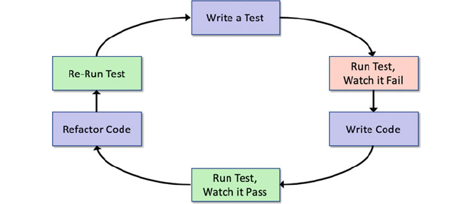
14.6.1 The TDD Cycle

There is a cycle to development when working in a TDD manner. The shortest form

of this cycle is the TDD mantra:

Red / Green / Refactor

Which relates to the unit testing suite of tools where it is possible to write a unit

test. Within tools such as PyCharm, when you run a pyunit or pytest test a Test

View is shown with Red indicating that a test failed or Green indicating that the test

passed. Hence Red/Green, in other words write the test and let it fail, then

implement the code to ensure it passes. The last part of this mantra is Refactor

which indicates once you have it working make the code cleaner, better, ﬁtter by

Refactoring it. Refactoring is the process by which the behaviour of the system is

not changed but the implementation is altered to improve it.

The full TDD cycle is shown by the following diagram which highlights the test

ﬁrst approach of TDD:

The TDD mantra can be seen in the TDD cycle that is shown above and

described in more detail below:

1. Write a single test.

2. Run the test and see it fail.

3. Implement just enough code to get the test to pass.

4. Run the test and see it pass.

5. Refactor for clarity and deal with any issue of reuse etc.

6. Repeat for next test.

172 14 Introduction to Testing

14.6.2 Test Complexity

The aim is to strive for simplicity in all that you do within TDD. Thus, you write a

test that fails, then do just enough to make that test pass (but no more). Then you

refactor the implementation code (that is change the internals of the unit under test)

to improve the code base. You continue to do this until all the functionality for a

unit has been completed. In terms of each test, you should again strive for simplicity

with each test only testing one thing with only a single assertion per test (although

this is the subject of a lot of debate within the TDD world).

14.6.3 Refactoring

The emphasis on refactoring within TDD makes it more than just testing or Test

First Development. This focus on refactoring is really a focus on (re)design and

incremental improvement. The tests provide the speciﬁcation of what is needed as

well as the veriﬁcation that existing behaviour is maintained, but refactoring leads

to better design software. Thus, without refactoring TDD is not TDD!

14.7 Design for Testability

Testability has a number of facets

• Conﬁgurability. Set up the object under test to an appropriate conﬁguration for

the test

• Controllability. Control the input (and internal state)

• Observability. Observe its output

• Veriﬁability. That we can verify that output in an appropriate manner.

14.7.1 Testability Rules of Thumb

If you cannot test code then change it so that you can!

If your code is difﬁcult to validate then change it so that it isn’t!

Only one concrete class should be tested per Unit test and then Mock the Rest!

If you code is hard to reconﬁgure to work with Mocks then make it so that you code

can use Mocks!

Design your code for testability!

14.6 Test Driven Development 173

14.8 Online Resources

See the following online resources for more information on testing and Test Driven

Development (TDD).

•

https://www.test-institute.org/Introduction _To_Software_Testing.php

Introduction to Software Testing.

•

https://en.wikibooks.org/wiki/Introduction_to_Software_Engineering/Testing

Introduction to software Testing wiki book.

•

https://en.wikipedia.org/wiki/Test-driven_development Test Driven Develop-

ment wikipedia page.

•

http://agiledata.org/essays/tdd.html an introduction to Test Driven Development.

•

https://medium.freecodecamp.org/learning-to-test-with-python-997ace2d8abe a

simple introduction to TDD with Python.

•

http://butunclebob.com/ArticleS.UncleBob.TheThreeRulesOfTdd Robert Mart-

ins three rules for TDD.

•

http://butunclebob.com/ArticleS.UncleBob.TheBowlingGameKata The Bowling

Game Kata which presents a worked example of how TDD can be used to create a

Ten Pin Bowls scoring keeping application.

14.9 Book Resources

• The Art of Software Testing, G. J. Myers, C. Sandler and T. Badgett, John Wiley

& Sons, 3rd Edition (Dec 2011), 1118031962.

174 14 Introduction to Testing

Chapter 15

PyTest Testing Framework

15.1 Introduction

There are several testing frameworks available for Python, although only one,

unittest comes as part of the typical Python installation. Typical libraries include

Unit test, (which is available within the Python distribution by default) and

PyTest.

In this chapter we will look at PyTest and how it can be used to write unit tests in

Python for both functions and classes.

15.2 What Is PyTest?

PyTest is a testing library for Python; it is currently one of the most popular Python

testing libraries (others include unittest and doctest). PyTest can be used for various

levels of testing, although its most common application is as a unit testing

framework. It is also often used as a testing framework within a TDD based

development project. In fact, it is used by Mozilla and Dropbox as their Python

testing framework.

PyTest offers a large number of features and great ﬂexibility in how tests are

written and in how set up behaviour is deﬁned. It automatically ﬁnds test based on

naming conventions and can be easily integrated into a range of editors and IDEs

including PyCharm.

J. Hunt, Advanced Guide to Python 3 Programming,

Undergraduate Topics in Computer Science,

https://doi.org/10.1007/978-3-030-25943-3_15

175

15.3 Setting Up PyTest

You will probably need to set up PyTest so that you can use it from within your

environment. If you are using the PyCharm editor, then you will need to add the

PyTest module to the current PyCharm project and tell PyCharm that you want to

use PyTest to run all tests for you.

15.4 A Simple PyTest Example

Something to Test

To be able to explore PyTest we ﬁrst need something to test; we will therefore

deﬁne a simple Calculator class. The calculator keeps a running total of the

operations perfor med; it allo ws a new value to be set and then this value can be

added to, or subtracted from, that accumulated total.

def __init__(self):

self.current = 0

self.total = 0

def set(self, value):

self.current = value

def add(self):

self.total += self.current

def sub(self):

self.total -= self.current

def total(self):

return self.total

class Calculator:

Save this class into a ﬁle called calculator.py.

Writing a Test

We will now create a very simple PyTest unit test for our Calculator class. This

test will be deﬁned in a class called test_calculator.py.

You will need to import the calculator class we wrote above into your

test_calculator.py ﬁle (remember each ﬁle is a module in Python).

176 15 PyTest Testing Framework

The exact import statement will depend on where you placed the calculator ﬁle

relative to the test class. In this case the two ﬁles are both in the same directory and

so we can write:

from calculator import Calculator

We will now deﬁne a test, the test should be pre-ﬁxed with test_ for PyTest to

ﬁnd them. In fact PyTest uses several conventions to ﬁnd tests, which are:

• Search for test_*.py or *_test.py ﬁles.

• From those ﬁles, collect test items:

– test_preﬁxed test functions,

– test_preﬁxed test methods inside Test preﬁxed test classes (without

an__init__method).

Note that we keep test ﬁles and the ﬁles containing the code to be tested separate;

indeed in many cases they are kept in different directory structures. This means that

there is not chance of developers accidentally using tests in production code etc.

Now we will add to the ﬁle a function that deﬁnes a test. We will call the

function test_add_one; it needs to start with test_ due to the above con-

vention. However, we have tried to make the rest of the function name descriptive,

so that its clear what it is testing. The function deﬁnition is given below:

from calculator import Calculator

def test_add_one():

calc = Calculator()

calc.set(1)

calc.add()

assert calc.total == 1

The test function creates a new instance of the Calculator class and then

calls several methods on it; to set up the value to add, then the call to the add()

method itself etc.

The ﬁnal part of the test is the assertion. The assert veriﬁes that the behaviour

of the calculator is as expected. The PyTest assert statement works out what is

being tested and what it should do with the result—including adding information to

be added to a test run report. It avoids the need to have to learn a load of

assertSomething type methods (unlike some other testing frameworks).

Note that a test without an assertion is not a test; i.e. it does not test anything.

Many IDEs provide direct support for testing frameworks including PyCharm.

For example, PyCharm will now detect that you have written a function with an

assert statement in it and add a Run Test icon to the grey area to the left of the

15.4 A Simple PyTest Example 177

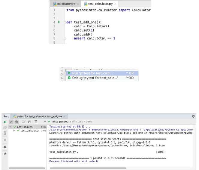
editor. This can be seen in the following picture where a green arrow has been

added at line 4; this is the ‘Run Test’ button:

The developer can click on the green arrow to run the test. They will then be

presented with the Run menu that is preconﬁgured to use PyTest for you:

If the developer now selects the Run option; this will use the PyTest runner to

execute the test and collect information about what happened and present it in a

PyTest output view at the bottom of the IDE:

Here you can see a tree in the left-hand panel that currently holds the one test

deﬁned in the test_calculator.py ﬁle. This tree shows whether tests have

passed or failed. In this case we have a green tick showing that the test passed.

To the right of this tree is the main output panel which shows the results of

running the tests. In this case it shows that Py Test ran only one test and that this was

the test_add_one test which was deﬁned in test_calculator.py and that

1 test passed.

If you now change the assertion in the test to check to see that the result is 0 the

test will fail. When run, the IDE display will update accordingly.

The tree in the left-hand pane now shows the test as failed while the right-hand

pane provides detailed information about the test that failed including where in the

test the failed assertion was deﬁned. This is very helpful when trying to debug test

failures.

178 15 PyTest Testing Framework

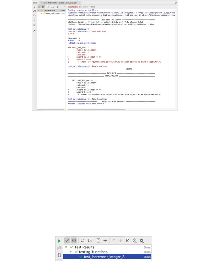
15.5 Working with PyTest

Testing Functions

We can test standalone functions as well as classes using PyTest. For example, given the

function increment below (which merely adds one to any number passed into it):

def increment(x):

return x + 1

We can write a PyTest test for this as follows:

def test_increment_integer_3():

assert increment(3) == 4

The only real difference is that we have not had to make an instance of a class:

Organising Tests

Tests can be grouped together into one or more ﬁles; PyTest will search for all ﬁles

following the naming convention (ﬁle names that either start or end with ‘test’)in

speciﬁed locations:

• If no arguments are speciﬁed when PyTest is run then the search for suitably

named test ﬁles starts from the testpaths environment variable (if conﬁg-

ured) or the current direc tory. Alternatively, command line arguments can be

used in any combination of directories or ﬁlenames etc.

15.5 Working with PyTest 179

• PyTest will recursively search down into sub directories, unless they

match norecursedirs environment variable.

• In those directories, it will search for ﬁles that match the naming conven-

tions test_*.py or *_test.py ﬁles.

Tests can also be arranged within test ﬁles into Test classes. Using test classes

can be helpful in grouping tests together and managing the setup and tear down

behaviours of separate groups of tests. However, the same effect can be achieved by

separating the tests relating to different functions or classes into different ﬁles.

Test Fixtures

It is not uncommon to need to run some behaviour before or after each test or

indeed before or after a group of tests. Such behaviours are deﬁned within what is

commonly known as test ﬁxtures.

We can add speciﬁc code to run:

• at the beginning and end of a test class module of test code (setup_mo dule/

teardown_module)

• at the beginning and end of a test class (setup_class/teardown_class) or using the

alternate style of the class level ﬁxtures (setup/teardown)

• before and after a test function call (setup_function/teardown_function)

• before and after a test method call (setup_method/teardown_method)

To illustrate why we might use a ﬁxture, let us expand our Calculator test:

def test_initial_value():

calc = Calculator()

assert calc.total == 0

def test_add_one():

calc = Calculator()

calc.set(1)

calc.add()

assert calc.total == 1

def test_subtract_one():

calc = Calculator()

calc.set(1)

calc.sub()

assert calc.total == -1

def test_add_one_and_one():

calc = Calculator()

calc.set(1)

calc.add()

calc.set(1)

calc.add()

assert calc.total == 2

180 15 PyTest Testing Framework

We now have four tests to run (we could go further but this is enough for now).

One of the issues with this set of tests is that we have repeated the creation of the

Calculator object at the start of each test. While this is not a problem in itself it

does result in duplicated code and the possibility of future issues in terms of

maintenance if we want to change the way a calculator is created. It may also not be

as efﬁcient as reusing the Calculator object for each test.

We can however, deﬁne a ﬁxture that can be run before each individual test

function is executed. To do this we will write a new function and use the

pytest.ﬁxture decorator on that function. This marks the function as being

special and that it can be used as a ﬁxture on an individual function.

Functions that require the ﬁxture should accept a reference to the ﬁxture as an

argument to the individual test function. For example, for a test to accept a ﬁxture

called calculator; it should have an argument with the ﬁxture name, i.e.

calculator. This name can then be used to access the object returned. This is

illustrated below:

import pytest

from calculator import Calculator

@pytest.fixture

def calculator():

"""Returns a Calculator instance"""

return Calculator()

def test_initial_value(calculator):

assert calculator.total == 0

def test_add_one(calculator):

calculator.set(1)

calculator.add()

assert calculator.total == 1

def test_subtract_one(calculator):

calculator.set(1)

calculator.sub()

assert calculator.total == -1

def test_add_one_and_one(calculator):

calculator.set(1)

calculator.add()

calculator.set(1)

calculator.add()

assert calculator.total == 2

15.5 Working with PyTest 181

In the above code, each of the test funct ions accepts the calculator ﬁxture

that is used to instantiate the Calculator object. We have therefore de-dupli-

cated our code; there is now only one piece of code that deﬁnes how a calculator

object should be created for our tests. Note each test is supplied with a completely

new instance of the Calculator object; there is therefore no chance of one test

impacting on another test.

It is also considered good practice to add a docstring to your ﬁxtures as we have

done above. This is because PyTest can produce a list of all ﬁxtures available along

with their docstrings. From the command line this is done using:

> pytest fixtures

The PyTest ﬁxtures can be applied to functions (as above), classes, modules,

packages or sessions. The scope of a ﬁxture can be indicated via the (optional)

scope parameter to the ﬁxture decorator. The default is “function” which is why

we did not need to specify anything above. The scope determines at what point a

ﬁxture should be run. For example, a ﬁxture with ‘session’ scope will be run once

for the test session, a ﬁxture with module scope will be run once for the module

(that is the ﬁxture and anything it generates will be shared across all tests in the

current module), a ﬁxture with class scope indicates a ﬁxture that is run for each

new instance of a test class created etc.

Another p arameter to the ﬁxture dec orator is autouse which if set to True will

activate the ﬁxture for all tests that can see it. If it is set to False (which is the default) then

an explicit reference in a test function (or method etc.) is required to activate the ﬁxture.

If we add some additional ﬁxtures to our tests we can see when they are run:

@pytest.fixture

def calculator():

"""Returns a Calculator instance"""

print('calculator fixture')

return Calculator()

import pytest

from calculator import Calculator

ue)

@pytest.fixture(scope='session', autouse=True)

def session_scope_fixture():

print('session_scope_fixture')

@pytest.fixture(scope='module',autouse=True)

@pytest.fixture(scope='class',autouse=Tr

def class_scope_fixture():

print('class_scope_fixture')

def module_scope_fixture():

print('module_scope_fixture')

182 15 PyTest Testing Framework

If we run this version of the tests, then the output shows when the various

ﬁxtures are run:

session_scope_fixture

odule_scope_fixture

class_scope_fixture

calculator fixture

.class_scope_fixture

calculator fixture

.class_scope_fixture

calculator fixture

.class_scope_fixture

calculator fixture

Note that higher scoped ﬁxtures are instantiated ﬁrst.

15.6 Parameterised Tests

One common requirement of a test to run the same tests multiple times with several

different input values. This can greatly reduce the number of tests that must be

deﬁned. Such tests are referred to as parametrised tests; with the parameter values

for the test speciﬁed using the @pytest.mark.parametrize decorator.

def test_initial_value(calculator):

assert calculator.total == 0

def test_add_one(calculator):

calculator.set(1)

calculator.add()

assert calculator.total == 1

def test_subtract_one(calculator):

calculator.set(1)

calculator.sub()

assert calculator.total == -1

def test_add_one_and_one(calculator):

calculator.set(1)

calculator.add()

calculator.set(1)

calculator.add()

assert calculator.total == 2

15.5 Working with PyTest 183

This illustrates setting up a parametrised test for the Calculator in which two

input values are added together and compared with the expected result. Note

that the parameters are named in the decorator and then a list of tuples is used to

deﬁne the values to be used for the parameters. In this case the test_

calculator_add_operation will be run tw o passing in 3, 1 and 4 and then

passing in 3, 2 and 5 for the parameters input1, input2 and expected

respectively.

Testing for Exceptions

You can write tests that verify that an exception was raised. This is useful as testing

negative behaviour is as important as testing positive behaviour. For example, we

might want to verify that a particular exception is raised when we attempt to

withdraw money from a bank account which will take us over our overdraft limit.

To verify the presence of an exception in PyTest use the with statement and

pytest.raises. This is a context manager that will verify on exit that the

speciﬁed exception was raised. It is used as follows:

ith pytest.raises(accounts.BalanceError):

current_account.withdraw(200.0)

Ignoring Tests

In some cases it is useful to write a test for functionality that has not yet been

implemented; this may be to ensure that the test is not forgotten or because it helps

to docum ent what the item under test should do. However, if the test is run then the

test suite as a whole will fail because the test is running against behaviour that has

yet to be written.

@pytest.mark.parametrize decorator.

@pytest.mark.parametrize('input1,input2,expected', [

(3, 1, 4),

(3, 2, 5),

])

def test_calculator_add_operation(calculator, input1,

input2,

expected):

calculator.set(input1)

calculator.add()

calculator.set(input2)

calculator.add()

assert calculator.total == expected

184 15 PyTest Testing Framework

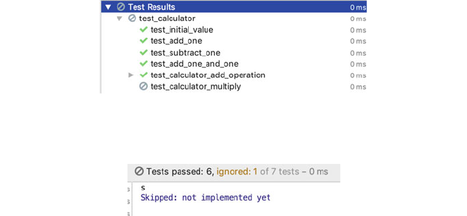
One way to address this problem is to decorate a test with the @pytest.-

mark.skip decorator:

@pytest.mark.skip(reason='not implemented yet')

def test_calculator_multiply(calculator):

calculator.multiply(2, 3)

assert calculator.total == 6

This indicates that PyTest should record the presence of the test but should not

try to execute it. PyTest will then note that the test was skipped, for example in

PyCharm this is shown using a circle with a line through it.

It is generally considered best practice to provide a reason why the test has been

skipped so that it is easier to track. This information is also available when PyTest

skips the test:

15.7 Online Resources

See the following online resources for information on PyTest:

•

http://pythontesting.net/framework/PyTest/PyTest-introduction/PyTest

introduction.

•

https://github.com/pluralsight/intro-to-PyTest An example based introduction to

PyTest.

•

https://docs.pytest.org/en/latest/PyTest home page.

•

https://docs.pytest.org/en/latest/#documentation PyTest documentation.

15.8 Exercises

Create a simple Calculator class that can be used for testing purposes. This

simple calculator can be used to add, subtract, multiple and divide numbers.

15.6 Parameterised Tests 185

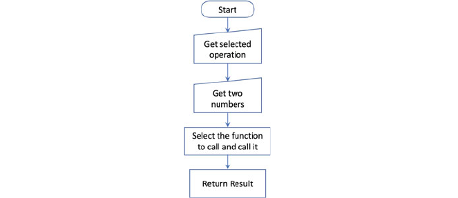
This will be a purely command driven application that will allow the user to

specify

• the operation to perform and

• the two numbers to use with that operation.

The Calculator object will then return a result. The same object can be used

to repeat this sequence of steps. This general behaviour of the Calculator is

illustrated below in ﬂow chart form:

You should also provide a memory function that allows the current result to be

added to or subtracted from the current memory total. It should also be possible to

retrieve the value in memory and clear the memory.

Next write a PyTest set of tests for the Calculator class.

Think about what tests you need to write; remember you can’t write tests for

every value that might be used for an operation; but consider the boundaries, 0, −1,

1, −10, +10 etc.

Of course you also need to consider the cumulative effect of the behaviour of the

memory feature of the calculator; that is multiple memory adds or memory sub-

tractions and combinations of these.

As you identify tests you may ﬁnd that you have to update your implementation

of the Calculator class. Have you taken into account all input options, for

example dividing by zero—what should happen in these situations.

186 15 PyTest Testing Framework

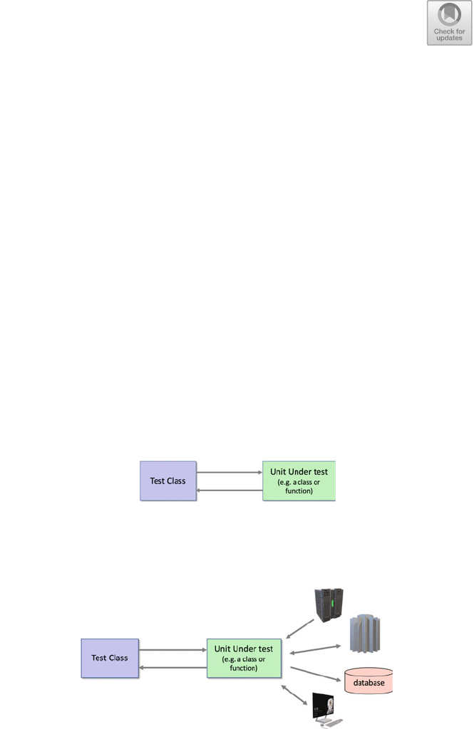
Chapter 16

Mocking for Testing

16.1 Introduction

Testing software systems is not an easy thing to do; the functions, objects, methods etc.

That are involved in any program can be complex things in their own right. In many

cases they depend on and interact with other functions, methods and objects; very few

functions and methods operate in isolation. Thus the success of failure of a function or

method or the overall state of an object is dependent on other program elements.

However, in general it is a lot easier to test a single unit in isolation rather than to

test it as part of a larger more complex system. For example, let us take a Python

class as a single unit to be tested. If we can test this class on its own we only have to

take into account the state of the classes object and the behaviour deﬁned for the

class when writing our test and determining appropriate outcomes.

However, if that class interacts with external systems such as external services,

databases, third party software, data sources etc. Then the testing process becomes

more complex:

J. Hunt, Advanced Guide to Python 3 Programming,

Undergraduate Topics in Computer Science,

https://doi.org/10.1007/978-3-030-25943-3_16

187

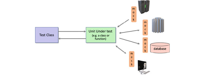
It may now be necessary to verify data updates made to the database, or information

sent to a remote service etc. to con ﬁrm that the operation of a class’s object is

correct. This makes not only the software being tested more complex but it also

makes the tests themselves more complex. This means that there is greater chance

that the test will fail, that the tests will contain bugs or issues themselves and that

the test will be harder for someone to understand and maintain. Thus a common

objective when writing unit tests or subsystem tests is to be able to test elements/

units in isolation.

The question is how to do this when a function or method relies on other

elements?

The ke y to decoupling functions, methods and objects from other program or

system elements is to use mocks. These mocks can be used to decouple one object

rom another, one function from another and one system from another; thereby

simplifying the testing environment. These mocks are only intended to be used for

testing purposes, for example the above scenario could be simpliﬁed by mocking

out each of the external systems as shown below:

Mocking is not a Python speciﬁc concept and there are many mocking libraries

available for may different languages. However, in this chapter we will be focussing

on the unites.mock library which has been part of the standard Python distribution

since Python 3.3.

16.2 Why Mock?

A useful ﬁrst question to consider with regard to mocking, in software testing, is

‘Why mock?’. That is, why bother with the concept of a mock in the ﬁrst place;

why not test with the real thing?

There are several answers to this, some of which are discussed below:

188 16 Mocking for Testing

Testing in isolation is easier. As mentioned in the introduction, testing a unit

(whether that is a class, a function, a module etc.) is easier in isolation then when

dependent on external classes, functions, modules etc.

The real thing is not available. In many cases it is necessary to mock out part

of a system or an interface to another system because the real thing is just not

available. This could be for several reasons including that it has not been developed

yet. In the natural course of software development some parts of a system are likely

to be developed and ready for testing before other parts. If one part relies on another

part for some element of its operation then the system that is not yet available can

be mocked out. In other situati ons the development team or test team may not have

access to the real thing. This may because it is only available within a production

context. For example, if a software development house is developing one subsys -

tem it may not have access to another subsystem as it is proprietary and only

accessible once the software has been deployed within the client organisation.

Real elements can be time consuming. We want our tests to run as quickly as

possible and certainly within a Continuous Integration (CI) environment we want

them to run fast enough that we can repeatedly test a system throughout the day. In

some situations the real thing may take a signiﬁcant amount of time to process the

test scenario. As we want to test our own code we may not be worried about

whether a system outside of our control operates correctly or not (at least at this

level of testing; it may still be a concern for integration and system testing). We can

therefore improve the response times of our tests if we mock out the real system and

replace it with a mock that provides much faster response times (possibly because it

uses canned responses).

The real thing takes time to set up. In a Continuous Integration

(CI) environment, new builds of a system are regularly and repeatedly tested (for

example whenever a change is made to their codebase). In such situations it may be

necessary to conﬁgure and deploy the ﬁnal system to a suitable environment to

perform appropriate tests. If an external system is time consuming to conﬁgure,

deploy and initialise it may be more effective to mock that system out.

Difﬁcult to emulate certain situations. It can be difﬁcult within a test scenario

to emulate speciﬁc situations. These situations are often related to error or excep-

tional circumstances that should never happen within a correctly functioning

environment. However, it may well be necessary to validate that if such a situation

does occur, then the software can deal with that scenario. If these scanners are

related to how external (the u nit under test) system fail or operate incorrectly then it

may be necessary to mock out these systems to be able to generate the scenarios.

We want repeatable tests. By their very nature when you run a test you either

want it to pass or fail each time it is run with the same inputs. You certainly do not

want tests that pass sometimes and fail other times. This mean that there is no

conﬁdence in the tests and people often start ignoring failed tests. This situa tion can

16.2 Why Mock? 189

happen if the data provided by systems that a test depends on do not supply

repeatable data. This can happen for several different reason but a common cause is

because they return real data. Such real data may be subject to change, for example

consider a system that uses a data feed for the current exchange rate between funds

and dollars. If the associated test conﬁrms that a trade when priced in dollars is

correctly converted to funds using the current exchange rate then that test is likely

to generate a different result every time it is run. In this situation it would lie better

to mock out the current exchange rate service so that a ﬁxed/known exchange rate is

used.

The Real System is not reliable enough. In some cases the real system may not

be reliable enough itself to allow for repeatable tests.

The Real System may not allo w tests to be repeated. Finally, the real system

may not allow tests to be easily repeated. For example, a test which involves

lodging a trade for a certain number of IBM shares with an Trade Order man-

agement system may not allow that trade, with those shares, for that customer to be

run several times (as it would then appear to be multiple trades). However, for the

purposes of testing we may want to test submitting such a trade in multipel different

scenarios, multiple times. It may therefore be necessary to mock out the real Order

Management System so that such tests can be written.

16.3 What Is Mocking?

The previous section gave several reasons to use mocks; the next thing to consider

then is what is a mock?

Mocks, including mock functions, methods and mock objects are things that:

• Possess the same interface as the real thing, whether they are mock functions,

methods or whole objects. They thus take the same range and types of

parameters and return similar information using similar types.

• Deﬁne behaviour that in some way represents/mimics real exemplar behaviour

but typically in very controlled ways. This behaviour may be hard coed, may

really on a set of rules or simpliﬁed behaviour; may be very simplistic or quiet

sophisticated in its own right.

They thus emulate the real system and from outside of the mock may actually

appear to be the real system.

In many cases the term mock is used to cover a range of different ways in which

the real thing can be emulated; each type of mock has its own characteristics. It is

therefore useful to distinguish the different types of mocks as this can help deter-

mine the style of mock to be adopted in a particular test situation.

190 16 Mocking for Testing

The are different types of Mock including:

• Test Stubs. A test stub is typically a hand coded function, method or object

used for testing purposes. The behaviour implemented by a test stub may rep-

resent a limited sub set of the functionality of the real thing.

• Fakes. Fakes typically provide addition functionalit y compared with a Test

Stub. Fakes may be considered to be a test speciﬁc version of the real thing,

such as an in memory database used for testing rather than the real database.

Such Fakes typically still have some limitations on their funct ionality, for

example when the tests are terminated all data is purged from the in memory

database rather than stored permanently on disk.

• Autogenerated Test Mocks. These are typically generated automatically using

a supporting framework. As part of the set up of the test the expect ations

associated with the test mock. These expectations may specify the results to

return for speciﬁc inputs as well as whether the test mock was called etc.

• Test Mock Spy. If we are testing a particular unit and it returns the correct result

we might decided that we do not need to consider the internal behaviour of the

unit. However, it is common to want to conﬁrm that the test mock was invoked

in the ay we expected. This helps verify the internal behaviour of the unit under

test. This can be done using a test mock spy. Such a test mock record s how

many times it was called and what the parameters used where (as well as other

information). The test can then interrogate the test mock to validate that it was

invoked as expected/as many times as expected/with the correct parameters etc.

16.4 Common Mocking Framework Concepts

As has been mentioned there are several mocking frameworks around for not only

Python but other languages such as Java, C# and Scala etc. All of these frameworks

have a common core behaviour. This behaviour allows a mock function, method or

object to be created based on the interface presented by the real thing. Of course

unlike languages such as C# and Java Python does not have a formal interface

concept; however this does not stop the mocking framework from still using the

same idea.

In general once a mock has been created it is possible to deﬁne how that mock

should appear to behave; in general this involves specifying the return result to use

for a function or method. It is also possible to verify that the mock has been invoked

as expected with the parameters expected.

The actual mock can be added to a test or a set of tests either programmatically

or via some form of decorator. In either case for the duration of the test the mock

will be used instead of the real thing.

16.3 What Is Mocking? 191

Assertions can then be used to verify the results returned by the unit under test

while mock speciﬁc methods are typically used to verify (spy on) the methods

deﬁned on the mock.

16.5 Mocking Frameworks for Python

Due to Python’s dynamic nature it is well suited to the construction of mock

functions, methods and objects. In fact there are several widely used mocking

frameworks available for Python including:

• unittest.mock The unittest.mock (included in the Python distribution from

Python 3.3 onwards). This is the default mocking library provided with Python

for creating mock objects in Python tests.

• pymox This is a widely used making framework. It is an open source frame-

work and has a more complete set of facilities for enforcing the inte rface of a

mocked class.

• Mocktest This is another popular mocking framework. It has its own DSL

(Domain Speciﬁc Language) to support mocking and a wide set of expectation

matching behaviour for mock objects.

In the rema inder of this chapter we will focus on the unittest.mock library as it

is provided as part of the standard Python distribution.

16.6 The unittest.mock Library

The standard Python mocking library is the unittest.mock library. It has been

included in the standard Python distribution since Python 3.3 and provides a simple

way to deﬁne mocks for unit tests.

The key to the unittest.mock library is the Mock class and its subclass

MagicMock. Mock and MagicMock objects can be used to mock functions,

methods and even whole classes. These mock objects can have canned responses

deﬁned so that when they are involved by the unit under test they will respond

appropriately. Existing objects can also have attributes or individual methods

mocked allo wing an object to be tested with a known state and speciﬁed behaviour.

To make it easy to work with mock objects, the library provides the

@unittest.moc k.patch() decorator. This decorator can be used to replace

real functions and objects with mock instances. The function behind the decorator

can also be used as a context manager allowing it to be used in with-as state-

ments providing for ﬁne grained control over the scope of the mock if required.

192 16 Mocking for Testing

16.6.1 Mock and Magic Mock Classes

The unittest.mock library provides the Mock class and the MagicMock

class. The Mock class is the base class for mock objects. The MagicMock class is

a subclass of the Mock class. It is called the MagicMock class as it provides

default implementations for several magic method such as .__len__(), .

__str__(),and.__iter__().

As a simple example consider the following class to be tested:

class SomeClass():

def _hidden_method(self):

return 0

def public_method(self, x):

return self.hidden

method() + x

This class deﬁnes two methods; one is intended as part of the public interface of the

class (the public_method()) and one it intended only for internal or private use

(the _hidden_method()). Notice that the hidden method uses the convention of

preceding its name by an underbar (‘_’).

Let us assume that we wish to test the behaviour of the public_method()

and want to mock out the _hidden_method().

We can do this by writing a test that will create a mock object and use this in

place of the real _hidden_method(). We could probably use either the Mock

class or the MagicMock class for this; however due to the additional functionality

provided by the MagicMock class it is common practice to use that class. We will

therefore do the same.

The test to be created will be deﬁned within a method within a test class. The

names of the test method and the test class are by convention descriptive and thus

will describe what is being tested, for example:

from unittest.mock import *

from unittest import TestCase

from unittest import main

class test_SomeClass_public_interface(TestCase):

def test_public_method(self):

test_object = SomeClass()

# Set up canned response on mock method

test_object._hidden_method = MagicMock(name =

'hidden_method')

test_object._hidden_method.return_value = 10

# Test the object

result = test_object.public_method(5)

self.assertEqual(15, result, 'return value from

public_method incorrect')

16.6 The unittest.mock Library 193

In this case note that the class being tested is instantiated ﬁrst. The MagicMock is

then instantiated and assigned to the name of the method to be mocked. This in

effect replaces that method for the test_object. The MagicMock. The

MagicMock object is given a name as this helps with treating any issues in the

report generated by the unites framework. Following this the canned response from

the mock version of the _hidden_method() is deﬁned; it will always return the

value 10.

At this point we have set up the mock to be used for the test and are now ready to

run the test. This is done in the next line where the public_method() is called

on the test_object with the parameter 5. The result is then stored.

The test then validates the result to ensure that it is correct; i.e. that the returned

value is 15.

Although this is a very simple example it illustrates how a method can be

mocked out using the MagicMock class.

16.6.2 The Patchers

The unittest.mock.patch() , unittest.mock.patch.object() and

unittest.patch.dict() decorators can be used to simplify the creat ion of

mock objects.

• The patch decorator takes a target for the patch and returns a MagicMock

object in its place. It can be used as a TastCase method or class decorator. As

a class de corator it decorates each test method in the class automatically. It can

also be used as a context manager via the with and with-as statements.

• The patch.object decorator can be provided with either two or three

arguments. When given three arguments it will replace the object to be patched,

with a mock for the given attribute/method name. When given two arguments

the object to be patched is given a default MagicMock object for the speci ﬁed

attribute/function.

• The patch.dict decorator patche s a dictionary or dictionary like object.

For example, we can rewrite the example presented in the previous section using

the @patch.object decorator to provides the mock object for the _hid-

den_method() (it returns a MagicMock linked to SomeClass):

194 16 Mocking for Testing

In the above code the _hidden_method() is replaced with a mock version for

SomeClass within the test_public_method() method. Note that the mock

version of the method is passed in as a parameter to the test method so that the

canned response can be speciﬁed.

You can also use the @patch() decorator to mock a function from a module.

For example, given some external module with a function api_call, we can

mock that function out using the @patch() decorator:

@patch('external_module.api_call')

def test_some_func(self, mock_api_call):

This uses patch() as a decorat or and passed the target object’ s path. The target

path was ‘external_module.a pi_call’ which consists of the module name and the

function to mock.

16.6.3 Mocking Returned Objects

In the examples looked at so far the results retur ned from the mock functions or

methods have been simple integers. However, in some cases the returned values

must themselves be mocked as the real system would return a complex object with

multiple attributes and methods.

The following examp le uses a MagicMock object to represent an object

returned from a mocked function. This object has two attributes, one is a response

code and the other is a JSON string. JSON stands for the JavaScript Object Notation

and is a commonly used format in web services.

class test_SomeClass_public_interface(TestCase):

@patch.object(SomeClass, '_hidden_method')

def test_public_method(self, mock_method):

# Set up canned response

mock_method.return_value = 10

# Create object to be tested

test_object = SomeClass()

result = test_object.public_method(5)

self.assertEqual(15, result, 'return value from

ublic_method incorrect')

16.6 The unittest.mock Library 195

In this example the function being tested is some_func() but some_func()

calls out to the mocked function external_module.api_call().

This mocked function returns a MagicMock object with a pre-speciﬁed

status_code and response. The assertions then validate that the object

returned by some_func() contai ns the correct status code and response.

16.6.4 Validating Mocks Have Been Called

Using unittest.mock it is possible to validate that a mocked function or

method was called appropriately using assert_called(), assert_-

called_with() or assert_called_once_with() depending on whether

the function takes parameters or not.

# Calls out to external API - which we want to mock

response = external_module.api_call()

return responseclass test_some_func_calling_api(TestCase):

class test_some_func_calling_api(TestCase):

@patch('external_module.api_call')

def test_some_func(self, mock_api_call):

# Sets up mock version of api_call

mock_api_call.return_value = MagicMock(status_code=200,

response=json.dumps({'key':'value'}))

# Calls some_func() that calls the (mock) api_call()

function

result = some_func()

# Check that the result returned from some_func() is

hat was expected

self.assertEqual(result.status_code, 200, "returned

status code is not 200")

self.assertEqual(result.response, '{"key": "value"}',

"response JSON incorrect")

import external_module

from unittest.mock import *

from unittest import TestCase

from unittest import main

import json

def some_func():

196 16 Mocking for Testing

The following version of the test_some_func_with_params() test

method veriﬁes that the mock api_call() function was called with the c orrect

parameter.

@patch('external_module.api_call_with_param')

def test_some_func_with_param(self, mock_api_call):

# Sets up mock version of api_call

mock_api_call.return_value = MagicMock(status_code=200,

response=json.dumps({'age': '23'}))

result = some_func_with_param('Phoebe')

# Check result returned from some_func() is what was

expected

self.assertEqual(result.response, '{age": "23"}', 'JSON

result incorrect')

# Verify that the mock_api_call was called with the correct

params

mock_api_call.api_call_with_param.assert_called_with('Phoebe')

If we wished to validate that it had only been called once we could use the

assert_called_once_with() method.

16.7 Mock and MagicMock Usage

16.7.1 Naming Your Mocks

It can be useful to give your mocks a name. The name is used when the mock

appears in test failure messages. The name is also propagated to attributes or

methods of the mock:

mock = MagicMock(name='foo')

16.7.2 Mock Classes

As well as mocking an individual method on a class it is possible to mock a whole

class. This is done by providing the patch() decorator with the name of the class

to patch (with no named attribute/method). In this case the while class is replaced

by a MagicMock object. You must then specify how that class should behave.

16.6 The unittest.mock Library 197

In this example the people.Person class has been mocked out. This class has a

method calculate_pay() which is being mocked here. The Payroll class

has a method generate_payslip() that expect s to be given a Person object.

It then uses the information provided by the person objects calculate_pay()

method to generate the string returned by the generate_payslip() method.

16.7.3 Attributes on Mock Classes

Attributes on a mock object can be easily deﬁned, for example if we want to set an

attribute on a mock object then we can just assign a value to the attribute:

import people

from unittest.mock import *

from unittest import TestCase

class MyTest(TestCase):

@patch('people.Person')

def test_one(self, MockPerson):

self.assertIs(people.Person, MockPerson)

instance = MockPerson.return_value

instance.age = 24

instance.name = 'Adam'

self.assertEqual(24, instance.age, 'age incorrect')

self.assertEqual('Adam', instance.name, 'name

incorrect')

In this case the attribute age and name have been added to the mock instance of

the people.Person class.

import people

from unittest.mock import *

from unittest import TestCase

from unittest import main

class MyTest(TestCase):

@patch('people.Person')

def test_one(self, MockPerson):

self.assertIs(people.Person, MockPerson)

instance = MockPerson.return_value

instance.calculate_pay.return_value = 250.0

payroll = people.Payroll()

result = payroll.generate_payslip(instance)

self.assertEqual('You earned 250.0', result, 'payslip

incorrect')

198 16 Mocking for Testing

If the attribute itself needs to be a mock object then all that is required is to

assign a MagicMock (or Mock) object to that attribute:

instance.address = MagicMock(name='Address')

16.7.4 Mocking Constants

It is very easy to mock out a constant; this can be done using the @patch()

decorator and proving the name of the constant and the new value to use. This value

can be a literal value such as 42 or ‘Hello’ or it can be a mock object itself (such as

a MagicMock object). For example:

@patch('mymodule.MAX_COUNT', 10)

def test_something(self):

# Test can now use mymodule.MAX

COUNT

16.7.5 Mocking Properties

It is also possible to mock Python properties. This is done again using the @patch

decorator but using the unittest.mock.PropertyMock class and the

new_callable param eter. For example:

@patch('mymoule.Car.wheels', new_callable=mock.PropertyMock)

def test_some_property(self, mock_wheels):

mock_wheels.return_value = 6

# Rest of test method

16.7.6 Raising Exceptions with Mocks

A very useful attribute that can be speciﬁed when a mock object is created is the

side_effect. If you set this to an exception class or instance then the exception

will be raised when the mock is called, for example:

mock = Mock(side_effect=Exception('Boom!'))

mock()

This will result in the Exception being raised when the mock() is invoked.

16.7 Mock and MagicMock Usage 199

16.7.7 Applying Patch to Every Test Method

If you want to mock out something for every test in a test class then you can

decorate the whole class rather than each individual method. The effect of deco-

rating the class is that the patch will be automatically applied to all test methods in

the class (i.e. To all methods starting with the word ‘test’). For example:

from unittest import TestCase

from unittest import main

@patch('people.Person')

class MyTest(TestCase):

def test_one(self, MockPerson):

self.assertIs(people.Person, MockPerson)

def test_two(self, MockSomeClass):

self.assertIs(people.Person, MockSomeClass)

def do_something(self):

return 'something'

import people

from unittest.mock import

In the above test class, the tests test_one and test_two are supplied with the

mock version of the Person class. However the do_something() method is

not affected.

16.7.8 Using Patch as a Context Manager

The patch function can be used as a context manager. This gives ﬁne grained

control over the scope of the mock object.

In the follow ing examp le the the test_one() method co ntains a with-as

statement that we used to patch (mock) the person class as MockPerson. This

mock class is only available within the with-as statemen t.

200 16 Mocking for Testing

16.8 Mock Where You Use It

The most common error made by people using the unittest.mock library is

mocking in the wrong place. The rule is that you must mock out where you are

going to use it; or to put it another way you must always mock the real thing where

it is imported into, not where it’s imported from.

16.9 Patch Order Issues

It is possible to have multiple patch decorators on a test method. However, the

order in which you deﬁne the patch decorators is signiﬁcant. The key to under-

standing what the order should be is to work backwards so that when the mocks are

passed into the test method they are presented to the right param eters. For example:

@patch('mymodule.sys')

@patch('mymodule.os')

@patch('mymodule.os.path')

def test_something(self,

mock_os_path,

mock_os,

mock_sys):

# The rest of the test method

import people

from unittest.mock import *

from unittest import TestCase

from unittest import main

class MyTest(TestCase):

def test_one(self):

with patch('people.Person') as MockPerson:

self.assertIs(people.Person, MockPerson)

instance = MockPerson.return_value

instance.calculate_pay.return_value = 250.0

payroll = people.Payroll()

result = payroll.generate_payslip(instance)

self.assertEqual('You earned 250.0', result,

'payslip incorrect')

16.7 Mock and MagicMock Usage 201

Notice that the last patch’s mock is passed into the second parameter passed to the

test_something() method (self is the ﬁrst parameter to all methods). In turn

the ﬁrst patch’s mock is passed into the last parameter. Thus the mocks are passed

into the test method in the reverse order to that which they are deﬁned in.

16.10 How Many Mocks?

An interesting question to consider is how many mocks should you use per test?

This is the subject or a lot of debate within the software testing community. The

general rules of thumb around this topic are given below, however it should be

borne in mind that these are guidelines rather than hard and fast rules.

• Avoid more than 2 or 3 mocks per test. You should avoid more than 2–3

mocks as the mocks themselves the get harder to manage. Many also consider

that if you need more then 2–3 mocks per test then there are probably some

underlying design issues that need to be considered. For example, if you are

testing a Python class then that class may have too many dependencies.

Alternatively the class may have too many responsibilities and should be broken

down into several independent classes; each with a distinct responsibility.

Another cause might be that the class’s behaviour may not be encapsulated

enough and that you are allowing other elements to interact with the class in

more informal ways (i.e. The interface between the class and other elements is

not c lean/exploit enough). The result is that it may be necessary to refactor your

class before progressing with your development and testing.

• Only Mock you Nearest Neighbour. You should only ever mock your nearest

neighbour whether that is a function, method or object. You should try to avoid

mocking dependencies of dependencies. If you ﬁnd yourself doing this then it

will become harder to conﬁgure, maintain, understand and develop. It is also

increasingly likely that you are testing the mocks rather than your own function,

method or class.

16.11 Mocking Considerations

The following provide some rules of thumb to consider when using mocks with

your tests:

• Don’t over mock—if you do then you can end up just testing the mocks

themselves.

202 16 Mocking for Testing

• Decide what to mock, typical examples of what to mock include those elements

that are not yet available, those elements that are not by default repeatable (such

as live data feeds) or those elements of the system that are time consuming or

complex.

• Decide where to mock such as the interfaces for the unit under test. You want

to test the unit so any interface it has with another system, function, class might

be a candidate for a mock.

• Decide when to mock so that you can determine the boundaries for the test.

• Decide how you will implement your mocks. For example you need to con-

sider which mocking framework(s) you will use or how to mock larger com-

ponents such as a database.

16.12 Online Resources

There is a great deal of information available on how to mock, when to mock and

what mock libraries to use, however the following provides useful starting points

for Python mocking:

•

https://docs.python.org/3/library/unittest.mock.html The Python Standard

Library documentation on the unitest.mock library.

•

https://docs.python.org/3/library/unittest.mock-examples.html A set of exam-

ples you can use to explore mocking using unites.mock.

•

https://pymox.readthedocs.io/en/latest/index.html Pymox is an alte rnative open

source mock object framework for Python.

•

http://gfxmonk.net/dist/doc/mocktest/doc mocktest its yet another mocking

library for Python.

16.13 Exercises

One of the reasons for mocking is to ensure that tests are repeatable. In this exercise

we will mock out the use of a random number generate to ensure that our tests can

be easily repeated.

The following program generates a deck of cards and randomly picks a card

from the deck:

16.11 Mocking Considerations 203

Each time the program is run a different card is picked, for example in two con-

secutive runs the following output is obtained:

You picked

13 of clubs

You picked

1 of hearts

We now want to write a test for the pick_a_card() function. You should mock

out the random.randint() function to do this.

import random

def create_suite(suite):

return [ (i, suite) for i in range(1, 14)]

def pick_a_card(deck):

print('You picked')

position = random.randint(0, 52)

print(deck[position][0], "of", deck[position][1])

return (deck[position])

# Set up the data

hearts = create_suite('hearts')

spades = create_suite('spades')

diamonds = create_suite('diamonds')

clubs = create_suite('clubs')

# Make the deck of cards

deck = hearts + spades + diamonds + clubs

# Randomly pick from the deck of cards

card = pick

card(deck)

204 16 Mocking for Testing

Part IV

File Input/Output

Chapter 17

Introduction to Files, Paths and IO

17.1 Introduction

The operat ing system is a critical part of any computer systems. It is comprised of

elements that manage the processes that run on the CPU, how memory is utilised

and managed, how peripheral devices are used (such as printers and scanners), it

allows the computer system to communicate with other systems and it also provide

support for the ﬁle system used.

The File System allows programs to permanently stor e data. This data can then

be retrieved by applications at a later date; potentially after the whole computer has

been shut down and restarted.

The File Management System is responsible for managing the creation, access

and modiﬁcation of the long term storage of data in ﬁles.

This data may be stored locally or remotely on disks, tapes, DVD drives, USB

drives etc.

Although this was not always the case; most modern operating systems organise

ﬁles into a hierarchical structure, usually in the form of an inverted tree. For

example in the following diagram the root of the directory structure is shown as ‘/’.

This root directory holds six subdirectories. In turn the Users subdirectory holds

3 further directories and so on:

J. Hunt, Advanced Guide to Python 3 Programming,

Undergraduate Topics in Computer Science,

https://doi.org/10.1007/978-3-030-25943-3_17

207

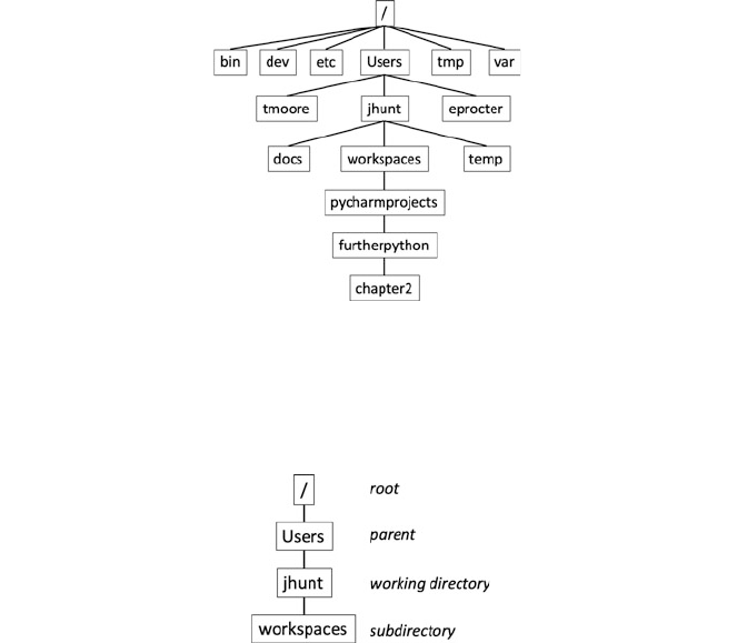
Each ﬁle is contained within a directory (also known as a folder on some operating

systems such as Windows). A directory can hold zero or more ﬁles and zero or

more directories.

For any give directory there are relationships with other directories as shown

below for the directory jhunt:

The root directory is the starting point for the hierarchical directory tree structure.

A child directory of a given directory is known as a subdirectory. The directory that

holds the given directory is known as the parent directory. At any one time, the

directory within which the program or user is currently working, is known as the

current working directory.

A user or a progra m can move around this directory structure as required. To do

this the user can typically either issue a series of commands at a terminal or

command window. Such as cd to change directory or pwd to print the working

directory. Alternatively Graphical User Interfaces (GUIs) to operating systems

usually include some form of ﬁle manager application that allows a user to view the

ﬁle structure in terms of a tree. The Finder program for the Mac is shown below

with a tree structure displayed for a pycharmprojects directory. A similar view

is also presented for the Windows Explorer program.

208 17 Introduction to Files, Paths and IO

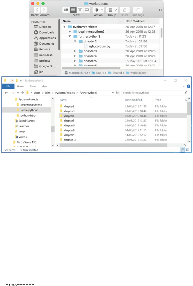
17.2 File Attributes

A ﬁle will have a set of attributes associated with it such as the date that it was

created, the date it was last updated/modiﬁed, how large the ﬁle is etc. It will also

typically have an attribute indicating who the owner of the ﬁle is. This may be the

creator of the ﬁle; however the ownership of a ﬁle can be changed either from the

command line or through the GUI interface. For example, on Linux and Mac OS X

the command chown can be used to change the ﬁle ownership.

It can also have other attributes which indicate who can read, write or execute

the ﬁle. In Unix style systems (such as Linux and Mac OS X) these access rights

can be speciﬁed for the ﬁle owner, for the group that the ﬁle is associated with and

for all other users.

The ﬁle owner can have rights speciﬁed for reading, writing and executing a ﬁle.

These are usually represented by the symbols ‘r’, ‘w’ and ‘x’ respectively. For

example the following uses the symbolic notation associated with Unix ﬁles and

indicates that the ﬁle owner is allowed to read, write and execute a ﬁle:

Here the ﬁrst dash is left blank as it is to do with special ﬁles (or directories), then

the next set of three characters represent the permissions for the owne r, the fol-

lowing set of three the permissions for all other users. As this example has rwx in

17.2 File Attributes 209

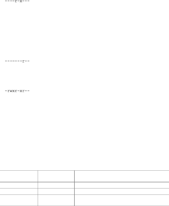
the ﬁrst group of three characters this indicates that the user can read ‘r’, write ‘w’

and execute ‘x’ the ﬁle. However the next six characters are all dashes indicating

that the group and all other users cannot access the ﬁle at all.

The group that a ﬁle belongs to is a group that can have any number of users as

members. A member of the group will have the access rights as indicated by the

group settings on the ﬁle. As for the owner of a ﬁle these can be to read, write or

execute the ﬁle. For example, if group members are allowed to read and execute a

ﬁle, then this would be shown using the symbolic notation as:

Now this example indicates that only members of the group can read and execute

the ﬁle; note that group members cannot write the ﬁle (they therefore cannot modify

the ﬁle).

If a user is not the owner of a ﬁle, nor a member of the group that the ﬁle is part

of, then their access rights are in the ‘everyone else’ category. Again this category

can have read, write or execute permissions. For example, using the symbolic

notation, if all users can read the ﬁle but are not able to do anything else, then this

would be shown as:

Of course a ﬁle can mix the above permissions together, so that an owner may be

allowed to read, write and execute a ﬁle, the group may be able to read and execute

the ﬁle but all other users can only read the ﬁle. This would be shown as:

In addition to the symbolic notation there is also a numeric notation that is used

with Unix style systems. The numeric notation uses three digits to represent the

permissions. Each of the three rightmost digits represents a different component of

the permissions: owner, group, and others.

Each of these digits is the sum of its component bits in the binary numeral

system. As a result, speciﬁc bits add to the sum as it is represented by a numeral:

• The read bit adds 4 to its total (in binary 100),

• The write bit adds 2 to its total (in binary 010), and

• The execute bit adds 1 to its total (in binary 001).

• This the following symboli c notations can be represented by an equivalent

numeric notation:

Symbolic

notation

Numeric

notation

Meaning

rwx—– 0700 Read, write, and execute only for owner

-rwxrwx— 0770 Read, write, and execute for owner and group

-rwxrwxrwx 0777 Read, write, and execute for owner, group and

others

210 17 Introduction to Files, Paths and IO

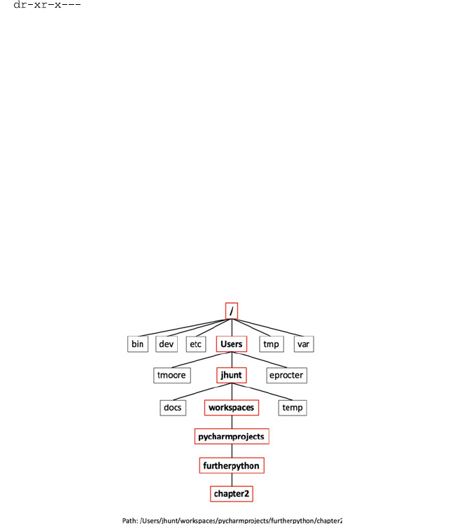
Directories have similar attributes and access rights to ﬁles. For example, the

following symbolic notation indicates that a directory (indicated by the ‘d’) has read

and execute permissions for the directory owner and for the group. Other users

cannot access this directory:

The permissions associated with a ﬁle or direc tory can be changed either using a

command from a terminal or command window (such as chmod which is used to

modify the permissions associated with a ﬁle or directory) or interactively using the

ﬁle explorer style tool.

17.3 Paths

A path is a particular combination of directories that can lead to a speciﬁc sub

directory or ﬁle.

This concept is important as Unix/Linux/Max OS X and Windows ﬁle systems

represent an inverted tree of directories and ﬁles., It is thus important to be able to

uniquely reference locations with the tree.

For example, in the following diagram the path /Users/jhunt/work-

spaces/pycharmprojects/furtherpython/chapter2 is highlighted:

A path may be absolute or relative. An absolute path is one which provides a

complete sequence of directories from the root of the ﬁle system to a speciﬁc sub

directory or ﬁle.

A relative path provides a sequence from the current working directory to a

particular subdirectory or ﬁle.

The absolute path will work wherever a program or user is cu rrently located

within the directory tree. However, a relative path may only be relevant in a speci ﬁc

location.

17.2 File Attributes 211

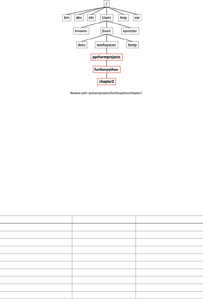
For example, in the following diagram, the relative path pycharmprojects/

furtherpython/chapter2 is only meaningful relative to the directory workspaces:

Note that an absolute path starts from the root directory (represented by ‘/’) where

as a relative path starts from a particular subdirectory (such as

pychamprojects).

17.4 File Input/Output

File Input/Output (often just referred to as File I/O) involves reading and writing

data to and from ﬁles. The data being written can be in different formats.

For example a common format used in Unix/Linux and Windows systems is the

ASCII text format. The ASCII format (or American Standard Code for Information

Interchange) is a set of codes that represent various characters that is widely used by

operating systems. The following table illustrates some of the ASCII character

codes and what they represent:

Decimal code Character Meaning

42 * Asterisk

43 + Plus

48 0 Zero

49 1 One

50 2 Two

51 3 Three

65 A Uppercase A

66 B Uppercase B

67 C Uppercase C

68 D Uppercase D

(continued)

212 17 Introduction to Files, Paths and IO

(continued)

Decimal code Character Meaning

97 a Lowercase a

98 b Lowercase b

99 c Lowercase c

100 d Lowercase d

ASCII is a very useful format to use for text ﬁles as they can be read by a wide

range of editors and browsers. These editors and browsers make it very easy to

create human readable ﬁles. However, programming languages such as Python

often use a different set of character encodings such as a Unicode character

encoding (such as UTF-8). Unicode is another standard for representing characters

using various codes. Unicode encoding systems offer a wider range of possible

character encodi ngs than ASCII, for example the latest version of Unicode in May

2019, Unicode 12.1, contains a repertoire of 137,994 characters covering 150

modern and historic scripts, as well as multiple symbol sets and emojis.

However, this means that it can be necessary to translate ASCII into Unicode

(e.g. UTF-8) and vice versa when reading and writing ASCII ﬁles in Python.

Another option is to use a binar y format for data in a ﬁle. The advantage of using

binary data is that there is little or no translation required from the internal repre-

sentation of the data used in the Python program into the format stored in the ﬁle. It

is also often more concise than an equivalent ASCII format and it is quicker for a

program to read and write and takes up less disk space etc. However, the down side

of a binary format is that it is not in an easily human readable format. It may also be

difﬁcult for other programs, particularly those written in other programming lan-

guages such as Java or C#, to read the data in the ﬁles.

17.5 Sequential Access Versus Random Access

Data can be read from (or indeed written to) a ﬁle either sequentially or via a

random access approach.

Sequential access to data in a ﬁle means that the program reads (or writes) data to

a ﬁle sequentially, starting at the beginning of a ﬁle and processing the data an item

at a time until the end of the ﬁle is reached. The read process only ever moves

forward and only to the next item of data to read.

Random Access to a data ﬁle means that the program can read (or write) data

anywhere into the ﬁle at any time. That is the program can posit ion itself at a

particular point in the ﬁle (or rather a pointer can be positioned within the ﬁle) and it

can then start to read (or write) at that point. If it is reading then it will read the next

data item relative to the pointer rather than the start of the ﬁle. If it is writing data

then it will write data from that point rather than at the end of the ﬁle. If there is

already data at that point in the ﬁle then it will be over written. This type of access is

17.4 File Input/Output 213

also known as Direct Access as the computer program needs to know where the

data is stored within the ﬁle and thus goes directly to that location for the data. In

some cases the location of the data is recorded in an index and thus is also known as

indexed access.

Sequential ﬁle access has advantages when a program needs to access infor-

mation in the same order each time the data is read. It is also is faster to read or

write all the data sequentially than via direct access as there is no need to move the

ﬁle pointer around.

Random access ﬁles however are more ﬂexible as data does not need to be

written or read in the order in which it is obtained. It is also possible to jump to just

the location of the data required and read that data (rather than needin g to

sequentially read through all the data to ﬁnd the data items of interest).

17.6 Files and I/O in Python

In the remainder of this section of the book we will explore the basic facilities

provided for reading and writing ﬁles in Python. We will also look at the underlying

streams model for ﬁle I/O. After this we will explore the widely used CSV and

Excel ﬁle formats and libraries available to support those. This section concludes by

exploring the Regular Expression facilities in Python. While this last topic is not

strictly part of ﬁle I/O it is often used to parse data read from ﬁles to screen out

unwanted information.

17.7 Online Resources

See the following online resources for information on the topics in this chapter:

•

https://en.wikipedia.org/wiki/ASCII Wikipedia page on ASCII.

•

https://en.wikipedia.org/wiki/Unicode Wikipedia page on Unicode.

•

https://en.wikipedia.org/wiki/UTF-8 Wikipedia page on UTF-8.

214 17 Introduction to Files, Paths and IO

Chapter 18

Reading and Writing Files

18.1 Introduction

Reading data from and writing data to a ﬁle is very common within many programs.

Python provides a large amount of support for working with ﬁles of various types.

This chapter introduces you to the core ﬁle IO functionality in Python.

18.2 Obtaining References to Files

Reading from, and writing to, text ﬁles in Python is relatively straightforward. The

built in open() function creates a ﬁle object for you that you can use to read and/

or write data from and/ or to a ﬁle.

The function requires as a minimum the name of the ﬁle you want to work with.

Optionally you can specify the access mode (e.g. read, write, append etc.). If you

do not specify a mode then the ﬁle is open in read-only mode. You can also specify

whether you want the interactions with the ﬁle to be buffered which can improve

performance by grouping data reads together.

The syntax for the open() function is

Where

• ﬁle_name indicates the ﬁle to be accessed.

• access_mode The access_mode determines the mode in which the ﬁle is

to be opened, i.e. read, write, append, etc. A complete list of possible values is

given below in the table. This is an optional parameter and the default ﬁle access

mode is read (r).

file_object = open(file_name, access_mode, buffering)

J. Hunt, Advanced Guide to Python 3 Programming,

Undergraduate Topics in Computer Science,

https://doi.org/10.1007/978-3-030-25943-3_18

215

• buffering If the buffering value is set to 0, no buffering takes place. If the

buffering value is 1, line buffering is performed while accessing a ﬁle.

The access_mode values are given in the following table.

The ﬁle object itself has several useful attributes such as

• ﬁle.closed returns True if the ﬁle has been closed (can no longer be

accessed because the close() method has been called on it).

• ﬁle.mode returns the access mode with which the ﬁle was opened.

• ﬁle.name The name of the ﬁle.

The ﬁle.close() method is used to close the ﬁle once you have ﬁnished with

it. This will ﬂush any unwritten information to the ﬁle (this may occur because of

buffering) and will close the reference from the ﬁle object to the actual underlying

operating system ﬁle. This is important to do as leaving a reference to a ﬁle open

can cause problems in larger applications as typically there are only a certain

number of ﬁle references possible at one time and over a long period of time these

Mode Description

r Opens a ﬁle for reading only. The ﬁle pointer is placed at the beginning of the ﬁle.

This is the default mode

rb Opens a ﬁle for reading only in binary format. The ﬁle pointer is placed at the

beginning of the ﬁle. This is the default mode

r+ Opens a ﬁle for both reading and writing. The ﬁle pointer placed at the beginning of

the ﬁle

rb+ Opens a ﬁle for both reading and writing in binary format. The ﬁle pointer placed at

the beginning of the ﬁle

w Opens a ﬁle for writing only. Overwrites the ﬁle if the ﬁle exists. If the ﬁle does not

exist, creates a new ﬁle for writing

wb Opens a ﬁle for writing only in binary format. Overwrites the ﬁle if the ﬁle exists. If

the ﬁle does not exist, creates a new ﬁle for writing

w+ Opens a ﬁle for both writing and reading. Overwrites the existing ﬁle if the ﬁle exists.

If the ﬁle does not exist, creates a new ﬁle for reading and writing

wb+ Opens a ﬁle for both writing and reading in binary format. Overwrites the existing ﬁle

if the ﬁle exists. If the ﬁle does not exist, creates a new ﬁle for reading and writing

a Opens a ﬁle for appending. The ﬁle pointer is at the end of the ﬁle if the ﬁle exists.

That is, the ﬁle is in the append mode. If the ﬁle does not exist, it creates a new ﬁle for

writing

ab Opens a ﬁle for appending in binary format. The

ﬁle pointer is at the end of the ﬁle if

the ﬁle exists. That is, the ﬁle is in the append mode. If the ﬁle does not exist, it

creates a new ﬁle for writing

a+ Opens a ﬁle for both appending and reading. The ﬁle pointer is at the end of the ﬁle if

the ﬁle exists. The ﬁle opens in the append mode. If the ﬁle does not exist, it creates a

new ﬁle for reading and writing

ab+ Opens a ﬁle for both appending and reading in binary format. The ﬁle pointer is at the

end of the ﬁle if the ﬁle exists. The ﬁle opens in the append mode. If the ﬁle does not

exist, it creates a new ﬁle for reading and writing

216 18 Reading and Writing Files

may all be used up resulting in future errors being thrown as ﬁles can no longer be

opened.

The following short code snippet illustrates the above ideas:

The output from this is:

18.3 Reading Files

Of course, having set up a ﬁle object we want to be able to either access the

contents of the ﬁle or write data to that ﬁle (or do both). Reading data from a text

ﬁle is supported by the read(), readline() and readlines() methods:

• The read() method This method will return the entire contents of the ﬁle as a

single string.

• The readline() method reads the next line of text from a ﬁle. It returns all

the text on one line up to and including the newline character. It can be used to

read a ﬁle a line at a time.

• The readlines() method returns a list of all the lines in a ﬁle, where each

item of the list represents a single line.

Note that once you have read some text from a ﬁle using one of the above

operations then that line is not read again. Thus using readlines() would result

in a further readlines() returning an empty list whatever the contents of the ﬁle.

The following illustrates using the readlines() method to read all the text in

a text ﬁle into a program and then print each line out in turn:

file = open('myfile.txt', 'r+')

print('file.name:', file.name)

print('file.closed:', file.closed)

print('file.mode:', file.mode)

file.close()

print('file.closed now:', file.closed)

file.name: myfile.txt

file.closed: False

file.mode: r+

file.closed now: True

file = open('myfile.txt', 'r')

lines = file.readlines()

for line in lines:

print(line, end='')

file.close()

18.2 Obtaining References to Files 217

Notice that within the for loop we have indicated to the print function that

we want the end character to be ''rather than a newline; this is because the line

string already possesses the newline character read from the ﬁle.

18.4 File Contents Iteration

As suggested by the previous example; it is very common to want to proces s the

contents of a ﬁle one line at a time. In fact Python makes this extremely easy by

making the ﬁle object support iteration. File iteration accesses each line in the ﬁle

and makes that line available to the for loop. We can therefore write:

It is also possible to use the list comprehension to provide a very concise way to

load and process lines in a ﬁle into a list. It is similar to the effect of readlines()

but we are now able to pre-process the data before creating the list:

18.5 Writing Data to Files

Writing a string to a ﬁle is supported by the write() method. Of course, the ﬁle

object we create must have an access mode that allows writing (such as 'w'). Note

that the write method does not add a newline character (represented as '\n') to the

end of the string—you must do this manually.

An example short program to write a text ﬁle is given below:

file = open('myfile.txt', 'r')

for line in file:

print(line, end='')

file.close()

file = open('

myfile.txt', 'r')

lines = [line.upper() for line in file]

file.close()

print(lines)

print('Writing file')

f = open('my-new-file.txt', 'w')

f.write('Hello from Python!!\n')

f.write('Working with files is easy...\n')

f.write('It is cool ...\n')

f.close()

218 18 Reading and Writing Files

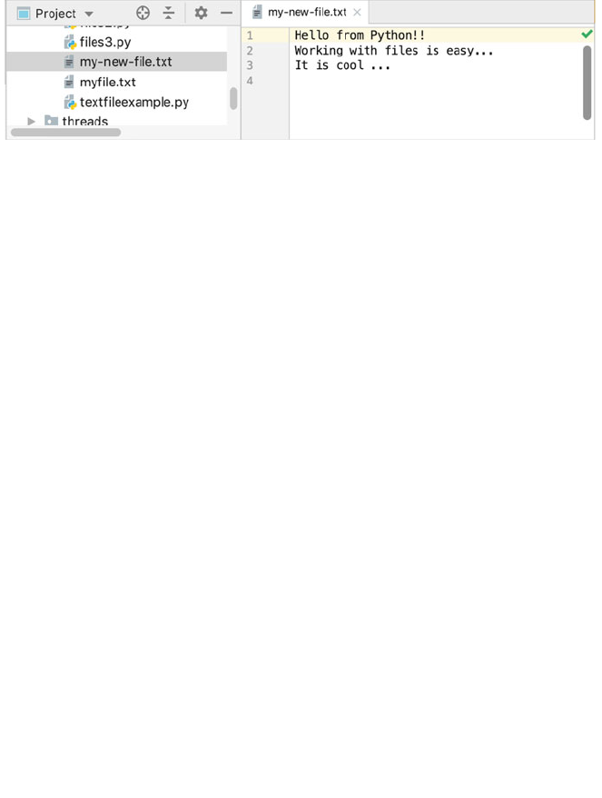
This creates a new ﬁle called my-new-ﬁle.txt. It then writes three strings to

the ﬁle each with a newline character on the end; it then closes the ﬁle.

The effect of this is to create a new ﬁle called myﬁle.txt with three lines in it:

18.6 Using Files and with Statements

Like several other types where it is imp ortant to shut down resources; the ﬁle object

class implements the Context Manager Protocol and thus can be used with the

with statement. It is therefore common to write code that will open a ﬁle using the

with as structure thus ensuring that the ﬁle will be closed when the block of code

is ﬁnished with, for example:

18.7 The Fileinput Module

In some situations, you may n eed to read the input from several ﬁles in one go. You

could do this by opening each ﬁle independently and then reading the contents and

appending that contents to a list etc. However, this is a common enough require-

ment that the ﬁleinput module provides a function ﬁleinput.input() that

can take a list of ﬁles and treat all the ﬁles as a single input signiﬁcantly simplifying

this process, for example:

ith open('my-new-file.txt', 'r') as f:

lines = file.readlines()

for line in lines:

print(line, end='')

ith fileinput.input(files=('spam.txt', 'eggs.txt')) as f:

for line in f:

process(line)

18.5 Writing Data to Files 219

Features provided by the ﬁleinput module include

• Return the name of the ﬁle currently being read.

• Return the integer “ﬁle descriptor” for the current ﬁle.

• Return the cumulative line number of the line that has just been read.

• Return the line number in the current ﬁle. Before the ﬁrst line has been read this

returns 0.

• A boolean function that indicates if the current line just read is the ﬁrst line of its

ﬁle

Some of these are illustrated below:

18.8 Renaming Files

A ﬁle can be renamed using the os.rename() function. This funct ion takes two

arguments, the current ﬁlename and the new ﬁlename. It is part of the Python os

module which provides methods that can be used to perform a range of

ﬁle-processing operations (such as renaming a ﬁle). To use the module, you will

ﬁrst need to import it. An example of using the rename function is given below:

18.9 Deleting Files

A ﬁle can be deleted using the os.remove() method. This method deletes the

ﬁle speciﬁed by the ﬁlename passed to it. Again, it is part of the os module and

therefore this must be imported ﬁrst:

ith fileinput.input(files=('textfile1.txt',

'textfile2.txt')) as f:

line = f.readline()

print('f.filename():', f.filename())

print('f.isfirstline():', f.isfirstline())

print('f.lineno():', f.lineno())

print('f.filelineno():', f.filelineno())

for line in f:

print(line, end='')

import os

os.rename('myfileoriginalname.txt',' myfilenewname.txt')

import os

os.remove('somefilename.txt')

220 18 Reading and Writing Files

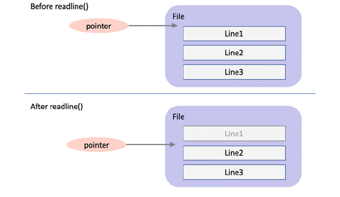
18.10 Random Access Files

All the examples presented so far suggest that ﬁles are accessed sequentially, with

the ﬁrst line read before the second and so on. Although this is (probably) the most

common approach it is not the only approach supported by Python; it is also

possible to use a random-access approach to the contents within a ﬁle.

To understand the idea of random ﬁle access it is useful to understand that we

can maintain a pointer into a ﬁle to indicate where we are in that ﬁle in terms of

reading or writing data. Before anything is read from a ﬁle the pointer is before the

beginning of the ﬁle and reading the ﬁrst line of text would for example, advance

the point to the start of the second line in the ﬁle etc. This idea is illustrated below:

When randomly accessing the contents of a ﬁle the programmer manually moves

the pointer to the location required and reads or writes text relative to that pointer.

This means that they can move around in the ﬁle reading and writing data.

The random-access aspect of a ﬁle is provided by the seek method of the ﬁle

object:

• ﬁle.seek (offset, whenc e) this method determines where the next read

or write operation (depending on the mode used in the open() call) takes

place.

In the above the offset parameter indicates the position of the read/ write pointer

within the ﬁle. The move can also be forwards or backwards (represented by a

negative offset).

The optional whence parameter indicates where the offset is relative to. The

values used for whence are:

18.10 Random Access Files 221

• 0 indicates that the offset is relative to start of ﬁle (the default).

• 1 means that the offset is relative to the current pointer position.

• 2 indicates the offset is relative to end of ﬁle.

Thus, we can move the point er to a position relative to the start of the ﬁle, to the

end of the ﬁle, or to the current position.

For example, in the following sample code we create a new text ﬁle and write a

set of characters into that ﬁle. At this point the pointer is positioned after the ‘z’ in

the ﬁle. However, we then use seek() to move the point to the 10th character in

the ﬁle and now write ‘Hello’, next we reposition the pointer to the 6th character

in the ﬁle and write out ‘BOO’. We then close the ﬁle. Finally, we read all the lines

from the ﬁle using a with as statement and the open() function and from this

we will see that the text is the ﬁle is now abcdefBOOjHELLOpqrstuvwxyz:

18.11 Directories

Both Unix like systems and Windows operating systems are hierarchical structures

comprising directories and ﬁles. The os module has several functions that can help

with creating, removing and altering directories. These include:

• mkdir() This function is used to create a directory, it takes the name of

the directory to create as a parameter. If the directory already

exists FileExistsError is raised.

• chdir() This function can be used to change the current working directory.

This is the directory that the application will read from/ write to by default.

• getcwd() This function returns a string representing the name of the current

working directory.

• rmdir() This function is used to remove/ delete a direc tory. It takes the name

of the directory to delete as a parameter.

• listdir() This function returns a list containing the names of the entri es in

the directory speciﬁed as a parameter to the function (if no name is given the

current directory is used).

f.close()

ith open('text.txt', 'r') as f:

for line in f:

print(line, end='')

f = open('text.txt', 'w')

f.write('abcdefghijklmnopqrstuvwxyz\n')

f.seek(10,0)

f.write('HELLO')

f.seek(6, 0)

f.write ('BOO')

222 18 Reading and Writing Files

A simple example illustrates the use of some of these functions is given below:

Note that ‘..’ is a short hand for the parent directory of the current directory and

‘.’ is short hand for the current directory.

An example of the type of output generated by this program for a speciﬁc set up

on a Mac is given below:

import os

print('os.getcwd(:', os.getcwd())

print('List contents of directory')

print(os.listdir())

print('Create mydir')

os.mkdir('mydir')

print('List the updated contents of directory')

print(os.listdir())

print('Change into mydir directory')

os.chdir('mydir')

print('os.getcwd(:', os.getcwd())

print('Change back to parent directory')

os.chdir('..')

print('os.getcwd(:', os.getcwd())

print('Remove mydir directory')

os.rmdir('mydir')

print('List the resulting contents of directory')

print(os.listdir())

os.getcwd(:

/Users/Shared/workspaces/pycharm/pythonintro/textfiles

List contents of directory

['my-new-file.txt', 'myfile.txt', 'textfile1.txt',

'textfile2.txt']

Create mydir

List the updated contents of directory

['my-new-file.txt', 'myfile.txt', 'textfile1.txt',

'textfile2.txt', 'mydir']

Change into mydir directory

os.getcwd(:

/Users/Shared/workspaces/pycharm/pythonintro/textfiles/mydir

Change back to parent directory

os.getcwd(:

/Users/Shared/workspaces/pycharm/pythonintro/textfiles

Remove mydir directory

List the resulting contents of directory

['my-new-file.txt', 'myfile.txt', 'textfile1.txt',

'textfile2.txt']

18.11 Directories 223

18.12 Temporary Files

During the execution of many applications it may be necessary to create a tem-

porary ﬁle that will be created at one point and deleted before the application

ﬁnishes. It is of course possible to manage such temporary ﬁles yourself however,

the tempﬁle module provides a range of facilities to simplify the creation and

management of these temporary ﬁles.

Within the tempﬁle module TemporaryFile, NamedTemporaryFile,

TemporaryDirectory, and SpooledTemporaryFile are high-level ﬁle

objects which provide automatic cleanup of temporary ﬁles and directories. These

objects implement the Context Manager Protocol .

The tempﬁle module also provides the lower-level function mkstemp() and

mkdtemp() that can be used to create temporary ﬁles that require the developer to

management them and delete them at an appropriate time.

The high-level feature for the tempﬁle module are:

• TemporaryFil e(mode=‘w+b’) Return an anonymous ﬁle-like object that

can be used as a temporary storage area. On completion of the managed context

(via a with statement) or destruction of the ﬁle object, the temporary ﬁle will

be removed from the ﬁlesystem. Note that by default all data is written to the

temporary ﬁle in binary format which is generally more efﬁcient.

• NamedTempora ryFile(mode=‘w+b’) This function operates exactly

as TemporaryFile() does, except that the ﬁle has s visible name in the ﬁle

system.

• SpooledTempo raryFile(max_size=0, mode=‘w+b’) This function

operates exactly as TemporaryFile() does, except that data is spooled in

memory until the ﬁle size exceeds max_size, or until the ﬁle’s ﬁleno

() method is called, at which point the contents are written to disk and oper-

ation proceeds as with TemporaryFile().

• TemporaryDir ectory(sufﬁx=None, preﬁx=None, dir=None)

This function creates a temporary directory. On completion of the context or

destruction of the temporary directory object the newl y created temporary

directory and all its contents are removed from the ﬁlesystem.

The lower level functions include:

• mkstemp() Creates a temporary ﬁle that is only readable or writable by the

user who created it.

• mkdtemp() Creates a temporary directory. The directory is readable, writable,

and searchable only by the creating user ID.

• gettempdir() Return the name of the directory used for temporary ﬁles.

This deﬁnes the default value for the default temporary directory to be used with

the other functions in this module.

An example of using the TemporaryFile funct ion is given below. This code

imports the tempﬁle module then prints out the default directory used for

224 18 Reading and Writing Files

temporary ﬁles. It then creates a TemporaryFile object and prints its name and

mode (the default mode is binary but for this ex ample we have overwritten this so

that plain text is used). We have then written a line to the ﬁle. Using seek we are

repositioning ourselves at the start of the ﬁle and then reading the line we have just

written.

The output from this when run on an Apple Mac is:

Note that the ﬁle name is ‘4’ and that the temporary directory is not a meaningful

name!

18.13 Working with Paths

The pathlib module provides a set of classes representing ﬁlesystem paths; that

is paths through the hierarchy of directories and ﬁles within an operating systems

ﬁle structure. It was introduced in Python 3.4. The core class in this module is the

Path class.

A Path object is useful because it provides operations that allow you to

manipulate and manage the path to a ﬁle or directory. The Path class also repli-

cates some of the operations available from the os module (such as mkdir,

rename and rmdir) which means that it is not necessary to work directly with the

os module.

A path object is created using the Path constructor function; this function

actually returns a speciﬁc type of Path depending on the type of operating system

being used such as a WindowsPath or a PosixPath (for Unix style systems).

import tempfile

print('tempfile.gettempdir():', tempfile.gettempdir())

temp = tempfile.TemporaryFile('w+')

print('temp.name:', temp.name)

print('temp.mode:', temp.mode)

temp.write('Hello world!')

temp.seek(0)

line = temp.readline()

print('line:', line)

tempfile.gettempdir():

/var/folders/6n/8nrnt9f93pn66ypg9s5dq8y80000gn/T

temp.name: 4

temp.mode: w+

line: Hello world!

18.12 Temporary Files 225

The Path() constructor takes the path to create for example ‘D:/mydir’ (on

Windows) or ‘/Users/user1/mydir’ on a Mac or ‘/var/temp’ on Linux

etc.

You can then use several different methods on the Path object to obtain infor-

mation about the path such as:

• exists() returns True of False depending on whether the path points to an

existing ﬁle or directory.

• is_dir() returns True if the path points to a directory. False if it refer-

ences a ﬁle. False is also returned if the path does not exist.

• is_ﬁle() returns True of the path points to a ﬁle, it returns False if the

path does not exist or the path references a directory.

• absolute() A Path object is considered absolute if it has both a root and (if

appropriate) a drive.

• is_absolute( ) returns a Boolean value indicating whether the Path is

absolute or not.

An example of using some of these methods is given below:

Sample output produced by this code snippet is:

There are also several methods on the Path class that can be used to create and

remove directories and ﬁles such as:

• mkdir() is used to create a directory path if it does not exist. If the path

already exists, then a FileExistsErr or is raised.

• rmdir() remove this directory; the d irectory must be empty otherwise an error

will be raised.

print('Create Path object for current directory')

p = Path('.')

print('p:', p)

print('p.exists():', p.exists())

print('p.is_dir():', p.is_dir())

print('p.is_file():', p.is_file())

print('p.absolute():', p.absolute())

from pathlib import Path

Create Path object for current directory

p: .

p.exists(): True

p.is_dir(): True

p.is_file(): False

p.absolute():

/Users/Shared/workspaces/pycharm/pythonintro/textfiles

226 18 Reading and Writing Files

• rename(targe t) rename this ﬁle or directory to the given target.

• unlink() removes the ﬁle referenced by the path object.

• joinpath(*ot her) appends elements to the path object e.g. path.joinpath(‘/

temp’).

• with_name(ne w_name) return a new path object with the name changed.

• The ‘/’ operator can also be used to create new path objects from existing paths

for example path/ ‘test’/ ‘output’ which would append the directories test and

out to the path object.

Two Path class methods can be used to obtain path objects representing key

directories such as the current working directory (the direc tory the program is

logically in at that point) and the home directory of the user running the program:

• Path.cwd() return a new path object representing the current directory.

• Path.home() return a new path object representing the user’s home

directory.

An example using several of the above features is given below. This example

obtains a path object representing the current working directory and then appends

‘text’ to this. The result path object is then checked to see if the path exists (on the

computer running the program), assuming that the path does not exist it is created

and the exists() method is rerun.

The effect of creating the directory can be seen in the output:

A very useful method in the Path object is the glob(pattern) method. This

method returns all elements within the path that meet the pattern speciﬁed.

For example path.glob(‘*.py’) will return all the ﬁles ending .py within

the current path.

p = Path.cwd()

print('Set up new directory')

newdir = p / 'test'

print('Check to see if newdir exists')

print('newdir.exists():', newdir.exists())

print('Create new dir')

newdir.mkdir()

print('newdir.exists():', newdir.exists())

Set up new directory

Check to see if newdir exists

newdir.exists(): False

Create new dir

newdir.exists(): True

18.13 Working with Paths 227

Note that ‘**/*.py’ would indicate the current directory and any sub directory.

For example, the following code will return all ﬁles where the ﬁle name ends with

‘.txt’ for a given path:

An example of the output generated by this code is:

Paths that reference a ﬁle can also be used to read and write data to that ﬁle. For

example the open() method can be used to open a ﬁle that by default allows a ﬁle

to be read:

• open(mode=‘r’) this can be used to open the ﬁle referenced by the path

object.

This is used below to read the contents of a ﬁle a line at a time (note that with

as statement is used here to ensure that the ﬁle represented by the Path is closed):

However, there are also some high-level methods available that allow you to

easily write data to a ﬁle or read data from a ﬁle. These include the Path methods

write_text and read_text methods:

• write_text(d ata) opens the ﬁle pointe d to in text mode and writes the

data to it and then closes the ﬁle.

• read_text() opens the ﬁle in read mode, reads the text and closes the ﬁle; it

then returns the contents of the ﬁle as a string.

print('-' * 10)

for file in path.glob('*.txt'):

print('file:', file)

print('-' * 10)

----------

file: my-new-file.txt

file: myfile.txt

file: textfile1.txt

file: textfile2.txt

----------

p = Path('mytext.txt')

ith p.open() as f:

print(f.readline())

228 18 Reading and Writing Files

These are used below

Which generates the following output:

18.14 Online Resources

See the following online resources for information on the topics in this chapter:

•

https://docs.python.org/3/tutorial/inputoutput.html for the Python Standard

Tutorial on ﬁle input and output.

•

https://pymotw.com/3/os.path/index.html for platform independent manipula-

tion of ﬁlenames.

•

https://pymotw.com/3/pathlib/index.html for information ﬁlesystem Path

objects.

•

https://pymotw.com/3/glob/index.html for ﬁlename pattern matching using glob.

•

https://pymotw.com/3/tempﬁle/index.html for temporary ﬁle system objects.

•

https://pymotw.com/3/gzip/index.html for information on reading and writing

GNU Zip ﬁles.

18.15 Exercise

The aim of this exercise is to explore the creation of, and access to, the contents of a

ﬁle.

You should write two programs, these programs are outlined below:

1. Create a program that will write todays date into a ﬁle – the name of the ﬁle can

be hard coded or supplied by the user. You can use the datetime.today()

dir = Path('./test')

print('Create new file')

newfile = dir / 'text.txt'

print('Write some text to file')

newfile.write_text('Hello Python World!')

print('Read the text back again')

rint(newfile.read_text())

print('Remove the file')

newfile.unlink()

Create new file

Write some text to file

Read the text back again

Hello Python World!

Remove the file

18.13 Working with Paths 229

function to obtain the current date and time. You can use the str() function to

convert this date time object into a string so that it can be written out to a ﬁle.

2. Create a second program to reload the date from the ﬁle and convert the string

into a date object. You can use the datetime.strptime() function to

convert a string into a date time object (see

https://docs.python.org/3/library/

datetime.html#datetime.datetime.strptime

for documentation on this function).

This functions takes a string containing a date and time in it and a second string

which deﬁnes the format expected. If you use the approach outlined in step 1

above to write the string out to a ﬁle then you should ﬁnd that the following

deﬁnes an appropriate format to parse the date_str so that a date time object

can be created:

atetime_object = datetime.strptime(date_str, '%Y-%m-%d

%H:%M:%S.%f')

230 18 Reading and Writing Files

Chapter 19

Stream IO

19.1 Introduction

In this chapter we will explore the Stream I/O model that under pins the way in

which data is read from and written to data sources and sinks. One example of a

data source or sink is a ﬁle but another might be a byte array.

This model is actually what sits underneath the ﬁle access mechanisms discussed

in the previous chapter.

It is not actually necessary to understand this model to be able to read and write

data to and from a ﬁle, however in some situations it is useful to have an under-

standing of this model so that you can modify the default behaviour when

necessary.

The remainder of this chapter ﬁrst introduces the Stream model, discusses

Python streams in general and then presents the classes provided by Python. It then

considers what is the actual effect of using the open() function presented in the last

chapter.

19.2 What is a Stream?

Streams are objects which serve as sources or sinks of data. At ﬁrst this concept can

seem a bit strange. The easiest way to think of a stream is as a conduit of data

ﬂowing from or into a pool. Some streams read data straight from the “source of the

data” and some streams read data from other streams. These latter streams then do

some “useful” processing of the data such as converting the raw data into a speciﬁc

format. The following ﬁgure illustrates this idea.

J. Hunt, Advanced Guide to Python 3 Programming,

Undergraduate Topics in Computer Science,

https://doi.org/10.1007/978-3-030-25943-3_19

231

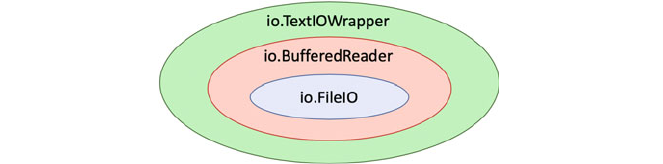
In the above ﬁgure the initial FileIO stream reads raw data from the actual data

source (in this case a ﬁle). The BufferedReader then buffers the data reading

process for efﬁciency. Finally the TextIOWrapper handles string encoding; that

is it converts strings from the typical ASCII representation used in a ﬁle into the

internal representation used by Python (which uses Unicode).

You might ask at this point why have a streams model at all; after all we read

and wrote data to ﬁles without needing to know about streams in the last chapter?

The answer is that a stream can read or write data to or from a source of data rather

than just from a ﬁle. Of course a ﬁle can be a source of data but so can a socket, a

pipe, a string, a web service etc. It is therefore a more ﬂexible data I/O model.

19.3 Python Streams

The Python io module provides Python’s main facilities for dealing with data input

and output. There are three main types of input/output these are text I/O, binary I/O

and raw I/.O. These categories can be used with various types of data source/sinks.

Whatever the category, each concrete stream can have a number of properties

such as being read-only, write-only or read-write. It can also support sequential

access or random access depending on the nature of the underlying data sink. For

example, reading data from a socket or pipe is inherently sequential where as

reading data from a ﬁle can be performed sequent ially or via a random access

approach.

Whichever stream is used however, they are aware of the type of data they can

process. Fo r example, attempting to supply a string to a binary write-only stream

will raise a TypeError. As indeed will presenting binary data to a text stream etc.

As suggested by this there are a number of different types of stream provided by

the Python io module and some of these are presented below:

232 19 Stream IO

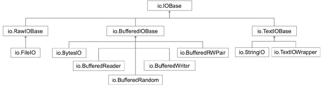
The abstract IOBase class is at the root of the stream IO class hierarchy. Below

this class are stream classes for unbuffered and buffered IO and for text oriented IO.

19.4 IOBase

This is the abstract base class for all I/O stream classes. The class provides many

abstract methods that subclasses will need to implement.

The IOBase class (and its subclasses) all support the iterator protocol. This

means that an IOBase object (or an object of a subclass) can iterate over the input

data from the underling stream.

IOBase also implements the Context Manager Protocol and therefore it can be

used with the with and with-as statements.

The IOBase class deﬁnes a core set of methods and attributes including:

• close() ﬂush and close the stream.

• closed an attribute indicating whether the stre am is close d.

• ﬂush() ﬂush the write buffer of the stream if applicable.

• readable() returns True if the stream can be read from.

• readline(siz e=-1) return a line from the stream. If size is speciﬁed at

most size bytes will be read.

• readline(hin t=-1) read a list of lines. If hint is speci ﬁed then it is used to

control the number of lines read.

• seek(offset[, whence]) This method moves the current the stream

position/pointer to the given offset. The meaning of the offset depends on the

whence parameter. The default value for whence is SEEK_SET.

• SEEK_SET or 0: seek from the start of the stream (the default); offset must

either be a number returned by TextIOBase.tell(), or zero. Any other offset value

produces undeﬁned behaviour.

• SEEK_CUR or 1: “seek” to the current position; offset must be zero, which is a

no-operation (all other values are unsupported).

• SEEK_END or 2: seek to the end of the stream; offset must be zero (all other

values are unsupported).

19.3 Python Streams 233

• seekable() does the stream support seek().

• tell() return the current stream position/pointer.

• writeable() returns true if data can be written to the stream.

• writelines(l ines) write a list of lines to the stream.

19.5 Raw IO/UnBuffered IO Classes

Raw IO or unbuffered IO is provided by the RawIOBase and FileIO classes.

RawIOBase This class is a subclass of IOBase and is the base class for raw

binary (aka unbuffered) I/O. Raw binary I/O typically provides low-level access to

an underlying OS device or API, and does not try to encapsulate it in high-level

primitives (this is the responsibi lity of the Buffered I/O and Text I/O classes that can

wrap a raw I/O stream). The class adds methods such as:

• read(size=-1 ) This method reads up to size bytes from the stream and

returns them. If size is unspeciﬁed or -1 then all available bytes are read.

• readall() This method reads and returns all available bytes within the

stream.

• readint(b) This method reads the bytes in the stream into a pre-allocated,

writable bytes-like object b (e.g. into a byte array). It returns the number of bytes

read.

• write(b) This method writes the data provided by b (a bytes -like object such

as a byte array) into the underlying raw stream.

FileIO The FileIO class represents a raw unbuffered binary IO stream linked

to an operating system level ﬁle. When the FileIO class is instantiated it can be

given a ﬁle name and the mode (such as ‘r’ or ‘w’ etc.). It can also be given a ﬂag to

indicate whether the ﬁle descriptor associated with the underlying OS level ﬁle

should be closed or not.

This class is used for the low-level reading of binary data and is at the heart of all

ﬁle oriented data access (although it is often wrapped by another stream such as a

buffered reader or writer).

19.6 Binary IO/Buffered IO Classes

Binary IO aka Buffered IO is a ﬁlter stream that wraps a lower level RawIOBase

stream (such as a FileIO stream). The classes implementing buffered IO all

extend the BufferedIOBase class and are:

BufferedReader When reading data from this object, a larger amount of data

may be requested from the underlying raw stream, and kept in an internal buffer.

The buffered data can then be returned directly on subsequent reads.

234 19 Stream IO

BufferedWriter When writing to this object, data is normally placed into an

internal buffer. The buffer will be written out to the underlying RawIOBase object

under various conditions, including:

• when the buffer gets too small for all pending data;

• when ﬂush() is called;

• when the BufferedWriter object is closed or destroyed.

BufferedRandom A buffered interface to random access streams. It sup-

ports seek() and tell() functionality.

BufferedRWPair A buffered I/O object combining two unidirectional

RawIOBase objects – one readable, the other writeable —into a single bidirectional

endpoint.

Each of the above classes wrap a lower level byte oriented stream class such as

the io.FileIO class, for example:

f = io.FileIO('data.dat’)

br = io.BufferedReader(f)

print(br.read())

This allows data in the form of bytes to be read from the ﬁle ‘data.dat’. You can

of course also read data from a different source, such as an in memory BytesIO

object:

binary_stream_from_file =

io.BufferedReader(io.BytesIO(b'starship.png'))

bytes = binary_stream_from_file.read(4)

print(bytes)

In this example the data is read from the BytesIO object by the

BufferedReader. The read() method is then used to read the ﬁrst 4 bytes, the

output is:

Note the ‘b’ in front of both the string ‘starship.png’ and the result ‘star’. This

indicates that the string literal should become a bytes literal in Python 3. Bytes

literals are always preﬁxed with ‘b’ or ‘B’; they produce an instance of the bytes

type instead of the str type. They may only contain ASCII characters.

The operations supported by buffered streams include, for reading:

• peek(n) return up to n bytes of data without advancing the stream pointer.

The number of bytes returned may be less or more than requested depending on

the amount of data available.

• read(n) return n bytes of data as bytes, if n is not supplied (or is negative) the

read all available data.

• readl(n) read up to n bytes of data using a single call on the raw data stream.

19.6 Binary IO/Buffered IO Classes 235

The operations supported by buffered writers include:

• write(bytes) writes the bytes-like data and returns the number of bytes

written.

• ﬂush() This method forces the bytes held in the buffer into the raw stream.

19.7 Text Stream Classes

The text stream classes are the TextIOBase class and its two subclasses

TextIOWrapper and StringIO.

TextIOBase This is the root class for all Text Stream classes. It provide s a

character and line based interface to Stream I/O. This class provides several

additional methods to that deﬁned in its parent class:

• read(size=-1 ) This method will return at most size characters from the

stream as a single string. If size is negative or None, it will read all remaining

data.

• readline(siz e=-1) This method will return a string representing the

current line (up to a newline or the end of the data whichever comes ﬁrst). If the

stream is already at EOF, an empty string is returned. If size is speciﬁed, at most

size characters will be read.

• seek(offset, [, whence]) change the stream position/pointer by the

speciﬁed offset. The optional whence parameter indicates where the seek

should start from:

– SEEK_SET or 0: (the default) seek from the start of the stream.

– SEEK_CUR or 1: seek to the current position; offset must be zero, which is a

no-operation.

– SEEK_END or 2: seek to the end of the stream; offset must be zero.

• tell() Returns the current stream position/pointer as an opaque number. The

number does not usually represent a number of bytes in the underlying binary

storage.

• write(s) This method will write the string s to the stream and return the

number of characters written.

TextIOWrapper. This is a buffered text stream that wraps a buffered binary

stream and is a direct subclass of TextIOBase. When a TextIOWrapper is

created there are a range of options available to control its behaviour:

io.TextIOWrapper(buffer, encoding=None, errors=None, newline=No

ne, line_buffering=False, write_through=False)

236 19 Stream IO

Where

• buffer is the buffered binary stream.

• encoding represents the text encoding used such as UTF-8.

• errors deﬁnes the error handling policy such as strict or ignore.

• newline controls how line endings are handled for example should they be

ignored (None) or represented as a linefeed, carriage return or a newline/carriage

return etc.

• line_buffering if True then ﬂush() is implied when a call to write

contains a newline character or a carriage return.

• write_throug h if True then a call to write is guaranteed not to be buffered.

The TextIOWrapper is wrapped around a lower level binary buffered I/O

stream, for example:

f = io.FileIO('data.txt')

br = io.BufferedReader(f)

text_stream = io.TextIOWrapper(br, 'utf-8')

StringIO This is an in memory stream for text I/O. The initial value of the buffer

held by the StringIO object can be provided when the instance is created, for

example:

This generates:

in_memory_text_stream <_io.StringIO object at 0x10fdfaee8>

to be or not to be that is the question

Note that the underlying buffer (represented by the string passed into the

StringIO instance) is discarded when the close() method is called.

The getvalue() method returns a string containing the entire contents of the

buffer. If it is called after the stream was closed then an error is generated.

19.8 Stream Properties

It is possible to query a stream to determine what types of operations it supports.

This can be done using the readable(), seekable() and writeable()

methods. For example:

in_memory_text_stream = io.StringIO('to be or not to be that is

the question')

print('in_memory_text_stream', in_memory_text_stream)

print(in_memory_text_stream.getvalue())

memory

text

stream.close()

19.7 Text Stream Classes 237

The output from this code snippet is:

19.9 Closing Streams

All opened streams must be closed. However, you can close the top level stream

and this will automatically close lower level streams, for example:

f = io.FileIO('data.txt’)

br = io.BufferedReader(f)

text_stream = io.TextIOWrapper(br, 'utf-8')

print(text_stream.read())

text_stream.close()

19.10 Returning to the open() Function

If streams are so good then why don’t you use them all the time? Well actually in

Python 3 you do! The core open function (and indeed the io.open() function)

both return a stream object. The actual type of object returned depends on the ﬁle

mode speciﬁed, whether buffering is being used etc. For example:

text_stream <_io.TextIOWrapper name='myfile.txt' encoding='utf-

8'>

text_stream.readable(): True

text_stream.seekable() True

text_stream.writeable() False

f = io.FileIO('myfile.txt')

br = io.BufferedReader(f)

text_stream = io.TextIOWrapper(br, encoding='utf-8')

print('text_stream', text_stream)

print('text_stream.readable():', text_stream.readable())

print('text_stream.seekable()', text_stream.seekable())

print('text_stream.writeable()', text_stream.writable())

text_stream.close()

238 19 Stream IO

When this short example is run the output is:

As you can see from the output, four different types of object have been returned

from the open() function. The ﬁrst is a TextIOWrapper, the second a

BufferedReader, the third a BufferedWriter and the ﬁnal one is a FileIO

object. This reﬂects the differences in the parameters passed into the open (0

function. For example, f1 references a io.TextIOWrapper because it must

encode (convert) the input text into Unicode using the UTF-8 encoding scheme.

While f2 holds a io.BufferedReader because the mode indicates that we want

to read binary data while f3 holds a io.BufferedWriter because the mode used

indicates we want to write binary data. The ﬁnal call to open returns a FileIO

because we have indicated that we do not want to buffer the data and thus we can

use the lowest level of stream object.

In general the following rules are applied to determine the type of object returned

based on the modes and encoding speciﬁed:

Class mode Buffering

FileIO binary no

BufferedReader ‘rb’ yes

BufferedWriter ‘wb’ yes

BufferedRandom ‘rb+’‘wb+’‘ab+’ yes

TextIOWrapper Any text yes

import io

# Text stream

f1 = open('myfile.txt', mode='r', encoding='utf-8')

print(f1)

# Binary IO aka Buffered IO

f2 = open('myfile.dat', mode='rb')

print(f2)

f3 = open('myfile.dat', mode='wb')

print(f3)

# Raw IO aka Unbufferedf IO

f4 = open('starship.png', mode='rb', buffering=0)

print(f4)

<_io.TextIOWrapper name='myfile.txt' mode='r' encoding='utf-8'>

<_io.BufferedReader name='myfile.dat'>

<_io.BufferedWriter name='myfile.dat'>

<_io.FileIO name='starship.png' mode='rb' closefd=True>

19.10 Returning to the open() Function 239

Note that not all mode combinations make sense and thus some combinations

will generate an error.

In general you don’ t therefore need to worry about which stream you are using

or what that stream does; not least because all the streams extend the IOBase class

and thus have a common set of methods and attributes.

However, it is useful to unders tand the implications of what you are doing so

that you can make better informed choices. For example, binary streams (that do

less processing) are faster than Unicode oriented streams that must convert from

ASCII into Unicode.

Also understanding the role of streams in Input and Output can also allow you to

change the source and destination of data without needing to re-write the whole of

your application. You can thus use a ﬁle or stdin for testing and a socket for reading

data in production.

19.11 Online Resources

See the following online resources for information on the topics in this chapter:

•

https://docs.python.org/3/library/io.html. This provides the Python Standard

Library guide to the core tools available for working with streams.

19.12 Exercise

Use the underl ying streams model to create an application that will write binary data

to a ﬁle. You can use the ‘b’ preﬁx to create a binary literal to be written, for

example b ‘Hello World’.

Next create another application to reload the binary data from the ﬁle and print it

out.

240 19 Stream IO

Chapter 20

Working with CSV Files

20.1 Introduction

This chapter introduces a module that supports the generation of CSV (or Comma

Separated Values) ﬁles.

20.2 CSV Files

The CSV (Comma Separated Values) format is the most common import and export

format for spreadsheets and databases. However, CSV is not a precise standard with

multiple different applications having different conventions and speciﬁc standards.

The Python csv module implements classes to read and write tabular data in

CSV format. As part of this it supports the concept of a dialect which is a CSV

format used by a speciﬁc application or suite of programs, for example, it supports

an Excel dialect.

This allows programmers to say, “write this data in the format preferred by

Excel,” or “read data from this ﬁle which was generated by Excel,” without

knowing the precise details of the CSV format used by Excel.

Programmers can also describe the CSV dialects understood by other applica-

tions or deﬁne their own special-purpose CSV dialects.

The csv module provides a range of functions including:

• csv.reader (csvﬁle, dialect='excel', ** fmtparams) Returns

a reader object which will iterate over lines in the given csvﬁle. An optional

dialect parameter can be given. This may be an instance of a subclass of the

Dialect class or one of the strings returned by the list_dialects()

function. The other optional fmtparams keyword arguments can be given to

override individual formatting parameters in the current dialect.

J. Hunt, Advanced Guide to Python 3 Programming,

Undergraduate Topics in Computer Science,

https://doi.org/10.1007/978-3-030-25943-3_20

241

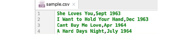
• csv.writer (csvﬁle, dialect='excel', **fmtparams) Returns

a writer object responsible for converting the user’s data into delimited strings

on the given csvﬁle. An optional dialect parameter provided. The fmtparams

keyword arguments can be given to override individual formatting parameters in

the current dialect.

• csv.list_dia lects() Return the names of all registered dialects. For

example on a Mac OS X the default list of dialects is ['excel', 'excel-tab', 'unix'].

20.2.1 The CSV Writer Class

A CSV Writer is obtained from the csv.writer() function. The csvwriter

supports two methods used to write data to the CSV ﬁle:

• csvwriter.wr iterow(row) Write the row parameter to the writer’s ﬁle

object, formatted according to the current dialect.

• csvwriter.wr iterows(rows) Write all elements in rows (an iterable of

row objects as described above) to the writer’s ﬁle object, formatted according

to the current dialect.

• Writer objects also have the following public attribute:

• csvwriter.di alect A read-only description of the dialect in use by the

writer.

The following program illustrates a simple use of the csv module which creates

a ﬁle called sample.csv.

As we have not speciﬁed a dialect, the default ‘excel’ dialect will be used. The

writerow() method is used to write each comma separate list of strings to the

CSV ﬁle.

print('Crearting CSV file')

ith open('sample.csv', 'w', newline='') as csvfile:

writer = csv.writer(csvfile)

writer.writerow(['She Loves You', 'Sept 1963'])

writer.writerow(['I Want to Hold Your Hand', 'Dec 1963'])

writer.writerow(['Cant Buy Me Love', 'Apr 1964'])

writer.writerow(['A Hard Days Night', 'July 1964'])

The resulting ﬁle can be viewed as shown below:

242 20 Working with CSV Files

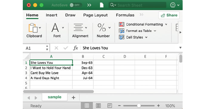
However, as it is a CSV ﬁle, we can also open it in Excel:

20.2.2 The CSV Reader Class

A CSV Reader object is obtained from the csv.reader() function. It imple-

ments the iteration protocol.

If a csv reader object is used with a for loop then each time round the loop it

supplies the next row from the CSV ﬁle as a list, parsed according to the current

CSV dialect.

Reader objects also have the following public attributes:

• csvreader.di alect A read-only description of the dialect in use by the

parser.

• csvreader.li ne_num The number of lines read from the source iterator.

This is not the same as the number of records returned, as records can span

multiple lines.

The following provides a very simple example of reading a CSV ﬁle using a csv

reader object:

print('Starting to read csv file')

with open('sample.csv', newline='') as csvfile:

reader = csv.reader(csvfile)

for row in reader:

print(*row, sep=', ')

print('Done Reading')

20.2 CSV Files 243

The output from this program, based on the sample.csv ﬁle created earlier is:

Starting to read csv file

She Loves You, Sept 1963

I Want to Hold Your Hand, Dec 1963

Cant Buy Me Love, Apr 1964

A Hard Days Night, July 1964

Done Reading

20.2.3 The CSV DictWriter Class

In many cases the ﬁrst row of a CSV ﬁle contains a set of names (or keys) that

deﬁne the ﬁelds within the rest of the CSV. That is the ﬁrst row gives meaning to

the columns and the data held in the rest of the CSV ﬁle. It is therefore very useful

to capture this information and to structure the data written to a CSV ﬁle or loaded

from a CSV ﬁle based on the keys in the ﬁrst row.

The csv.DictWriter returns an object that can be used to write values into

the CSV ﬁle based on the use of such named columns. The ﬁle to be used with the

DictWriter is provided when the class is instantiated.

import csv

with open('names.csv', 'w', newline='') as csvfile:

fieldnames = ['first_name', 'last_name', 'result']

writer = csv.DictWriter(csvfile, fieldnames=fieldnames)

writer.writeheader()

writer.writerow({'first_name': 'John',

'last_name': 'Smith',

'result' : 54})

writer.writerow({'first_name': 'Jane',

'last_name': 'Lewis',

'result': 63})

writer.writerow({'first_name': 'Chris',

'last_name': 'Davies',

'result' : 72})

Note that when the DictWriter is created a list of the keys must be provided

that are used for the columns in the CSV ﬁle.

The method writeheader() is then used to write the header row out to the

CSV ﬁle.

The method writerow() takes a dictionary object that has keys based on the

keys deﬁned for the DictW riter. These are then used to write data out to the

CSV (note the order of the keys in the dictionary is not important).

In the above examp le code the result of this is that a new ﬁle called names.csv

is created which can be opened in Excel:

Of course, as this is a CSV ﬁle it can also be opened in a plain text editor as well.

244 20 Working with CSV Files

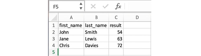
20.2.4 The CSV DictReader Class

As well as the csv.DictWriter there is a csv.DictReader. The ﬁle to be

used with the DictReader is provided when the class is instantiated. As with the

DictReader the DictWriter class takes a list of keys used to deﬁne the

columns in the CSV ﬁle. If the headings to be used for the ﬁrst row can be provided

although this is optional (if a set of keys are not provided, then the values in the ﬁrst

row of the CSV ﬁle will be used as the ﬁeldnames).

The DictReader class provides several useful features including the

ﬁeldnames property that contains a list of the keys/headings for the CSV ﬁle as

deﬁned by the ﬁrst row of the ﬁle.

The DictReader class also implements the iteration protocol and thus it can

be used in a for loop in which each row (after the ﬁrst row) is returned in turn as a

dictionary. The dictionary object representing each row can then be used to access

each column value based on the keys deﬁned in the ﬁrst row.

An example is shown below for the CSV ﬁle created earlier:

import csv

print('Starting to read dict CSV example')

with open('names.csv', newline='') as csvfile:

reader = csv.DictReader(csvfile)

for heading in reader.fieldnames:

print(heading, end=' ')

print('\n------------------------------')

for row in reader:

print(row['first_name'], row['last_name'],

row['result'])

print('Done')

20.2 CSV Files 245

This generates the following output:

Starting to read dict CSV example

first_name last_name result

------------------------------

John Smith 54

Jane Lewis 63

Chris Davies 72

Done

20.3 Online Resources

See the following online resources for information on the topics in this chapter:

•

https://docs.python.org/3/library/csv.html for the Python Standard documenta-

tion on CSV ﬁle reading and writing.

•

https://pymotw.com/3/csv/index.html for the Python Module of the Week page

on CSV ﬁles.

•

https://pythonprogramming.net/reading-csv-ﬁles-python-3 for a tutorial on

reading CSV ﬁles.

20.4 Exercises

In this exercise you will create a CSV ﬁle based on a set of transactions stored in a

current account.

1. To do this ﬁrst deﬁne a new Account class to represent a type of bank account.

2. When the class is instantiated you should provide the account number, the name

of the account holder, an opening balance and the type of account (which can be

a string representing 'current', 'deposit' or 'investment' etc.). This means that

there must be an __init__ method and you wi ll need to store the data within

the object.

3. Provide three instance methods for the Account; deposit(amount),

withdraw(amo unt) and get_balance(). The behaviour of these

methods should be as expected, deposit will increase the balance, withdraw

will decrease the balance and get_balance() returns the current balance.

Your Account class should also keep a history of the transactions it is involved

in.

A Transaction is a record of a deposit or withdrawal along with an amount.

Note that the initial amount in an account can be treated as an initial deposit.

246 20 Working with CSV Files

The history could be implemented as a list containing an ordered sequenc e to

transactions. A Transact ion itself could be deﬁned by a class with an action (deposit

or withdrawal) and an amount.

Each time a withdrawal or a deposit is made a new transaction record should be

added to a transaction history list.

Next provide a function (which could be called something like write_ac-

count_transactions_to_csv() ) that can take an account and then write

each of the transactions it holds out to a CSV ﬁle, with each transaction type and the

transaction amount separated by a comma.

The following sample application illustrates how this function might be used:

print('Starting')

acc = accounts.CurrentAccount('123', 'John', 10.05, 100.0)

acc.deposit(23.45)

acc.withdraw(12.33)

print('Writing Account Transactions')

write_account_transaction_to_csv('accounts.csv', acc)

print('Done')

The contents of the CSV ﬁle would then be:

20.4 Exercises 247

Chapter 21

Working with Excel Files

21.1 Introduction

This chapter introduces the openpyxl module that can be used when working

with Excel ﬁles. Excel is a software application developed by Microsoft that allows

users to work with spreadsheets. It is a very widely used tool and ﬁles using the

Excel ﬁle format are commonly encountered within many organisations. It is in

effect the industry standard for spreadsheets and as such is a very useful tool to have

in the developers toolbox.

21.2 Excel Files

Although CSV ﬁles are a convenient and simple way to handle data; it is very

common to need to be able to read or write Excel ﬁles directly. To this end there are

several libraries available in Python for this purpose. One widely used library is the

OpenPyXL library. This library was originally written to support access to Excel

2010 ﬁles. It is an open source project and is well documented.

The OpenPyXL library provides facilities for

• reading and writing Excel workbooks,

• creating/accessing Excel worksheets,

• creating Excel formulas,

• creating graphs (with support from additional modul es).

As OpenPyXL is not part of the standard Python distribution you will need to

install the library yourself using a tool such as Anaconda or pip (e.g. pip

install openpyxl). Alternatively, if you are using PyCharm you will be able

to add the OpenPyXL library to your project.

J. Hunt, Advanced Guide to Python 3 Programming,

Undergraduate Topics in Computer Science,

https://doi.org/10.1007/978-3-030-25943-3_21

249

21.3 The Openpyxl. Workbook Class

The key element in the OpenPyXL library is the Workbook class. This can be

imported from the module:

from openpyxl import Workbook

A new instance of the (in memory) Workbook can be created using the

Workbook class (note at this po int it is purely a structure within the Python

program and must be saved before an actual Excel ﬁle is created).

wb = Workbook()

21.4 The Openpyxl. WorkSheet Objects

A workbook is always created with at least one worksheet. You can get hold of the

currently active worksheet using the Workbook.active property:

ws = wb.active

You can create additional worksheets using the workbooks’ create_sheet

() method:

ws = wb.create_sheet('Mysheet')

You can access or update the title of the worksheet using the title proper ty:

ws.title = 'New Title'

The background colour of the tab holding this title is white by default. You can

change this providing an RRGGBB colour code to the worksheet.

sheet_properties.tabColor attribut e, for example:

ws.sheet_properties.tabColor = "1072BA"

21.5 Working with Cells

It is possible to access the cells within a worksheet. A cell can be accessed directly

as keys on the worksheet, for example:

ws['A1'] = 42

250 21 Working with Excel Files

cell = ws['A1']

This returns a cell object; you can obtain the value of the cell using the value

property, for example

print(cell.value)

There is also the Worksheet.cell() method. This provides access to cells

using row and column notation:

d = ws.cell(row=4, column=2, value=10)

A row of values can also be added at the current position within the Excel ﬁle

using append:

ws.append([1, 2, 3])

This will add a row to the Excel ﬁle containing 1, 2, and 3.

Ranges of cells can be accessed using slicing:

cell_range = ws['A1':'C2']

Ranges of rows or columns can also be obtained:

col = ws['C']

col_range = ws['C:D']

row10 = ws[10]

row_range = ws[5:10]

The value of a cell can also be an Excel formula such as

ws['A3'] = '=SUM(A1, A2)'

A workbook is actually only a structure in memory; it must be saved to a ﬁle for

permanent storage. These workbooks can be saved using the save() method. This

method takes a ﬁlename and writes the Workbook out in Excel format.

workbook = Workbook()

...

workbook.save('balances.xlsx')

21.6 Sample Excel File Creation Application

The following simple application creates a Workbook with two worksheets. It also

contains a simple Excel formula that sums the values held in to other cells:

21.5 Working with Cells 251

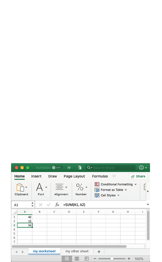
The Excel ﬁle generated from this can be viewed in Excel as shown below:

from openpyxl import Workbook

def main():

print('Starting Write Excel Example with openPyXL')

workbook = Workbook()

# Get the current active worksheet

ws = workbook.active

ws.title = 'my worksheet'

ws.sheet_properties.tabColor = '1072BA'

ws['A1'] = 42

ws['A2'] = 12

ws['A3'] = '=SUM(A1, A2)'

ws2 = workbook.create_sheet(title='my other sheet')

ws2['A1'] = 3.42

ws2.append([1, 2, 3])

ws2.cell(column=2, row=1, value=15)

workbook.save('sample.xlsx')

print('Done Write Excel Example')

if __name__ == '__main__':

main()

252 21 Working with Excel Files

21.7 Loading a Workbook from an Excel File

Of course, in many cases it is necessary not just to create Excel ﬁles for data export

but also to import data from an existing Excel ﬁle. This can be done using the

OpenPyXL load_workbook() function. This function opens the speciﬁed Excel

ﬁle (in read only mode by default) and returns a Workbook object.

from openpyxl import load_workbook

workbook = load_workbook(filename='sample.xlsx')

You can now access a list of sheets, their names, obtain the currently active sheet

etc. using properties provided by the workbook object:

• workbook.act ive returns the active worksheet object.

• workbook.she etnames returns the names (strings) of the worksheets in this

workbook.

• workbook.wor ksheets returns a list of worksheet objects.

The following sample application reads the Excel ﬁle created earlier in this

chapter:

from openpyxl import load_workbook

def main():

print('Starting reading Excel file using openPyXL')

workbook = load_workbook(filename='sample.xlsx')

print(workbook.active)

print(workbook.sheetnames)

print(workbook.worksheets)

print('-' * 10)

ws = workbook['my worksheet']

print(ws['A1'])

print(ws['A1'].value)

print(ws['A2'].value)

print(ws['A3'].value)

print('-' * 10)

for sheet in workbook:

print(sheet.title)

print('-' * 10)

cell_range = ws['A1':'A3']

for cell in cell_range:

print(cell[0].value)

print('-' * 10)

21.7 Loading a Workbook from an Excel File 253

print('Finished reading Excel file using openPyXL')

if __name__ == '__main__':

main()

The output from this application is illustrated below:

Starting reading Excel file using openPyXL

['my worksheet', 'my other sheet']

[<Worksheet "my worksheet">, <Worksheet "my other sheet">]

----------

=SUM(A1, A2)

----------

y worksheet

y other sheet

----------

=SUM(A1, A2)

----------

Finished reading Excel file using openPyXL

21.8 Online Resources

See the following online resources for information on the topics in this chapter:

•

https://openpyxl.readthedocs.io/en/stable for documentation on the OpenPyXL

Python to Excel library.

21.9 Exercises

Using the Account class that you created in the last chapter; write the account

transaction information to an Excel ﬁle instead of a CSV ﬁle.

To do this create a function called write_account_transaction_to_excel

() that takes the name of the Excel ﬁle and the account to store. The function should then

write the data to the ﬁle using the excel format.

254 21 Working with Excel Files

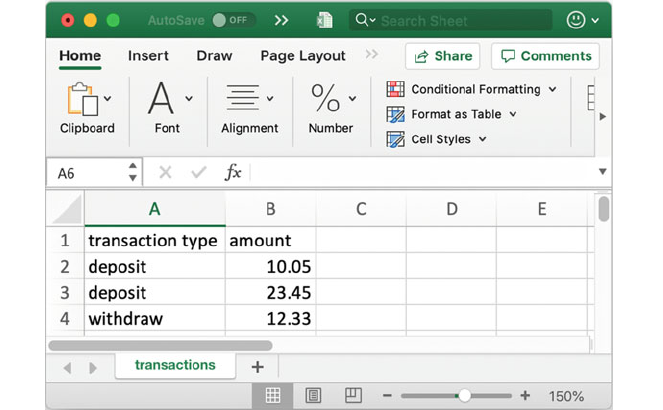
The following sample application illustrates how this function might be used:

print('Starting')

acc = accounts.CurrentAccount('123', 'John', 10.05, 100.0)

acc.deposit(23.45)

acc.withdraw(12.33)

print('Writing Account Transactions')

write_account_transaction_to_excel(‘accounts.xlsx’, acc)

print('Done')

The contents of the Excel ﬁle would then be:

21.9 Exercises 255

Chapter 22

Regular Expressions in Python

22.1 Introduction

Regular Express ion are a very powerful way of processing text while looking for

recurring patterns; they are often used with data held in plain text ﬁles (such as log

ﬁles), CSV ﬁles as well as Excel ﬁles. This chapter introduces regular expressions,

discusses the syntax used to deﬁne a regular expression pattern and presen ts the

Python re module and its use.

22.2 What Are Regular Expressions?

A Regular Expression (also known as a regex or even just re) is a sequence of

characters (letters, numbers and special characters) that form a pattern that can be

used to search text to see if that text contains sequences of characters that match the

pattern.

For example, you might have a pattern deﬁned as three characters followed by

three numbers. This pattern could be used to look for such a pattern in other strings.

Thus, the following strings either match (or contain) this pattern or they do not:

Abc123 Matches the pattern

A123A Does not match the pattern

123AAA Does not match the pattern

J. Hunt, Advanced Guide to Python 3 Programming,

Undergraduate Topics in Computer Science,

https://doi.org/10.1007/978-3-030-25943-3_22

257

Regular Expression are very widely used for ﬁnding information in ﬁles, for

example

• ﬁnding all lines in a log ﬁle associated with a speciﬁc user or a speci ﬁc

operation,

• for validating input such as checking that a string is a valid email address or

postcode/ZIP code etc.

Support for Regular Expressions is wide spread within programming languages

such as Java, C#, PHP and particularly Perl. Python is no exception and has the

built-in module re (as well as additional third-party modules) that suppor t Regular

Expressions.

22.3 Regular Expression Patterns

You can deﬁne a regular expression pattern using any ASCII character or number.

Thus, the string ‘John’ can be used to deﬁne a regex pattern that can be used to

match any other string that contains the characters ‘J’, ‘o’, ‘h’, ‘n’. Thus each of the

following strings will match this pattern:

• ‘John Hunt’

• ‘John Jones’

• ‘Andrew John Smith’

• ‘Mary Helen John’

• ‘John John John’

• ‘I am going to visit the John’

• ‘I once saw a ﬁlm by John Wayne’

But the following strings would not match the pattern:

• ‘Jon Davies’ in this case because the spelling of John is different.

• ‘john williams’ in this case because the capital J does not match the lowercase j.

• ‘David James’ in this case because the string does not contain the string John!

Regular expressions (regexs) use special characters to allow more complex patterns

to be described. For example, we can use the special characters ‘[]’ to deﬁne a set

of characters that can match. For example, if we want to indicate that the J may be a

capital or a lower-case letter then we can write ‘ [Jj]’—this indicates that either ‘J’ or

‘j’ can match the ﬁrst.

• [Jj]ohn

—this states that the pattern starts with either a capital J or a lowercase j

followed by ‘ohn’.

Now both ‘john williams’ and ‘John Williams’ will match this regex pattern.

258 22 Regular Expressions in Python

22.3.1 Pattern Metacharacters

There are several special characters (often referred to as metacharacters) that have a

speciﬁc meaning within a regex pattern, these are listed in the following table:

Character Description Example

[] A set of characters [a-d] characters in the sequence ‘a’ to

‘d’

\ Indicates a special sequence (can also

be used to escape special characters)

‘\d’ indicates the character should be

an integer

. Any character with the exception of

the newline character

‘J.hn’ indicates that there can be any

character after the ‘J’ and before the

‘h’

^ Indicates a string must start with the

following pattern

“^hello” indicates the string must start

with ‘hello’

$ Indicates a string must end with the

preceding pattern

“world$” indicates the string must end

with ‘world’

* Zero or more occurrences of the

preceding pattern

“Python*” indicates we are looking for

zero or more times Python is in a

string

+ One or more occurrences of preceding

pattern

“info+” indicates that we must ﬁnd

info in the string at least once

? Indicates zero or 1 occurrences of the

preceding pattern

“john?” indicates zero or one instances

of the ‘John’

{} Exactly the speciﬁed number of

occurrences

“John{3}” this indicates we expect to

see the ‘John’ in the string three times.

“X{1,2}” indicates that there can be

one or two Xs next to each other in the

string

| Either or “True|OK” indicates we are looking

for either True or OK

() Groups together a regular expression;

you can then apply another operator to

the whole group

“(abc|xyz){2}” indicates that we are

looking for the string abc or xyz

repeated twice

22.3.2 Special Sequences

A special sequence is a combination of a ‘\’ (backslash) followed by a character

combination which then has a special meaning. The following table lists the

common special sequences used in Regular Expressions:

22.3 Regular Expression Patterns 259

Sequence Description Example

\A Returns a match if the following characters are

at the beginning of the string

“\AThe” must start with ‘The’

\b Returns a match where the speciﬁed characters

are at the beginning or at the end of a word

“\bon” or “on\b” indicates a

string must start or end with

‘on’

\B Indicates that the following characters must be

present in a string but not at the start (or at the

end) of a word

r”\Bon” or r”on\B” must not

start or end with ‘on’

\d Returns a match where the string contains

digits (numbers from 0–9)

“\d”

\D Returns a match where the string DOES NOT

contain digits

“\D”

\s Returns a match where the string contains a

white space character

“\s*”

\S Returns a match where the string DOES NOT

contain a white space character

“\S”

\w Returns a match where the string contains any

word characters (characters from a to Z, digits

from 0–9, and the underscore _ character)

“\w”

\W Returns a match where the string DOES NOT

contain any word characters

“\W”

\Z Returns a match if the following characters are

present at the end of the string

“Hunt\Z”

22.3.3 Sets

A set is a sequence of characters inside a pair of square brackets which have speciﬁc

meanings. The following table provides some examples.

Set Description

[jeh] Returns a match where one of the speciﬁed characters (j, e or h) are present

[a–x] Returns a match for any lower-case character, alphabetically between a and x

[^zxc] Returns a match for any character EXCEPT z, x and c

[0123] Returns a match where any of the speciﬁed digits (0, 1, 2, or 3) are present

[0–9] Returns a match for any digit between 0 and 9

[0–9][0–9] Returns a match for any two-digit numbers from 00 and 99

[a–zA–Z] Returns a match for any character alphabetically between a and z or A and Z

260 22 Regular Expressions in Python

22.4 The Python re Module

The Python re module is the built-in module provided by Python for working with

Regular Expressions.

You might also like to examine the third party regex module (see

https://pypi.

org/project/regex

) which is backwards compatible with the default re module but

provides additional functionality.

22.5 Working with Python Regular Expressions

22.5.1 Using Raw Strings

An important point to note about many of the stri ngs used to deﬁne the regular

expression patterns is that they are preceded by an ‘r’ for example r'/bin/sh$'.

The ‘r’ before the string indicates that the string should be treated as a raw

string.

A raw string is a Python string in which all characters are treated as exactly that;

individual characters. It means that backslash (‘\’) is treat ed as a literal character

rather than as a special character that is used to escape the next character.

For example, in a standard string ‘ \n’ is treated as a special character repre-

senting a newline, thus if we wrote the following:

We will get as output:

However, if we preﬁx the string with an ‘r’ then we are telling Python to treat it as

a raw string. For example:

The output is now

This is important for regular expression as characters such as backslash (‘\’) are

used within patterns to have a special regular expression meaning and thus we do

not want Python to process them in the normal way.

s = 'Hello \n world'

print(s)

Hello

World

s = r'Hello \n world'

print(s)

Hello \n world

22.4 The Python re Module 261

22.5.2 Simple Example

The following simple Python program illustrates the basic use of the re module. It

is necessary to import the re module before you can use it.

When this program is run, we get the following output:

If we look at the code, we can see that the string that we are examining contains ‘john

williams’ and that the pattern used with this string indicates that we are looking for a

sequence of ‘J’ or ‘j’ followed by ‘ohn’. To perform this test we use the re.

search() function passing the regex pattern, and the text to test, as parameters.

This function returns either None (which is taken as meaning False by the If

statement) or a Match Object (which always has a Boolean value of True). As of

course ‘john’ at the start of text1 does match the pattern, the re.search()

function returns a match object and we see the ‘Match has been found’ message is

printed out.

Both the Match object and search() method will be described in more detail

below; however, this short program illustrates the basic operation of a Regular

Expression.

22.5.3 The Match Object

Match objects are returned by the search() and match() functions.

They always have a boolean value of True.

The functions match() and search() return None when there is no match

and a Match object when a match is found. It is therefore possible to use a match

object with an if statement:

import re

text1 = 'john williams'

pattern = '[Jj]ohn'

print('looking in', text1, 'for the pattern', pattern)

if re.search(pattern, text1):

print('Match has been found')

looking in john williams for the pattern [Jj]ohn

Match has been found

262 22 Regular Expressions in Python

Match objects support a range of methods and attributes including:

• match.re The regular expression object whose match() or search()

method produced this match instance.

• match.string The string passed to match() or search().

• match.start( [group]) / match.end([group]) Return the indices

of the start and end of the substring matched by group.

• match.group( ) returns the part of the string where there was a match.

22.5.4 The search() Function

The search() function searches the string for a match, and returns a Match

object if there is a match. The signature of the function is:

The meaning of the parameters are:

• pattern this is the regular expression pattern to be used in the matching

process.

• string this is the string to be searched.

• ﬂags these (optional) ﬂags can be used to modify the operation of the search.

The re module deﬁnes a set of ﬂags (or indicators) that can be used to indicate any

optional behaviours associated with the pattern. These ﬂags include:

Flag Description

re.IGNORECASE Performs case-insensitive matching

re.LOCALE Interprets words according to the current locale. This interpretation affects

the alphabetic group (\w and \W), as well as word boundary behavior(\b

and \B)

re.MULTILINE Makes $ match the end of a line (not just the end of the string) and makes

^ match the start of any line (not just the start of the string)

re.DOTALL Makes a period (dot) match any character, including a newline

re.UNICODE Interprets letters according to the Unicode character set. This ﬂag affects

the behavior of \w, \W, \b, \B

re.VERBOSE Ignores whitespace within the pattern (except inside a set [] or when

escaped by a backslash) and treats unescaped # as a comment marker

import re

atch = re.search(pattern, string)

if match:

process(match)

re.search(pattern, string, flags=0)

22.5 Working with Python Regular Expressions 263

If there is more than one match, only the ﬁrst occurrence of the match will be

returned:

In this case the output is

Another example of using the search() function is given below. In this case the

pattern to look for deﬁnes three alternative strings (that is the string must contain

either Beatles, Adele or Gorillaz):

In this case we generate the output:

22.5.5 The match() Function

This function attempts to match a regular expression pattern at the beginning of a

string. The signature of this function is given below:

import re

line1 = 'The price is 23.55'

containsIntegers = r'\d+'

if re.search(containsIntegers, line1):

print('Line 1 contains an integer')

else:

print('Line 1 does not contain an integer')

Line 1 contains an integer

import re

# Alternative words

usic = r'Beatles|Adele|Gorillaz'

request = 'Play some Adele'

if re.search(music, request):

print('Set Fire to the Rain')

else:

print('No Adele Available')

Set Fire to the Rain

re.match(pattern, string, flags=0)

264 22 Regular Expressions in Python

The parameters are:

• pattern this is the regular expression to be matched.

• string this is the string to be searched.

• ﬂags modiﬁer ﬂags that can be used.

The re.match() function returns a Match object on success, None on failure.

22.5.6 The Difference Between Matching and Searching

Python offers two different primitive operations based on regular expressions:

• match() checks for a match only at the beginning of the string,

• search() checks for a match anywhere in the string.

22.5.7 The ﬁndall() Function

The ﬁndall() function returns a list containing all matches. The signature of this

function is:

This function returns all non-overlapping matches of pattern in string ,asa

list of strings.

The string is scanned left -to-right, and matches are returned in the order

found. If one or more groups are present in the pattern, then a list of groups is

returned; this will be a list of tuples if the pattern has more than one group. If no

matches are found, an empty list is returned.

An example of using the ﬁndall() function is given below. This example

looks for a substring starting with two letters and followed by ‘ai’ and a single

character. It is applied to a sentence and returns only the sub string ‘Spain’ and

‘plain’.

re.findall(pattern, string, flags=0)

import re

str = 'The rain in Spain stays mainly on the plain'

results = re.findall('[a-zA-Z]{2}ai.', str)

print(results)

for s in results:

print(s)

22.5 Working with Python Regular Expressions 265

The output from this program is

22.5.8 The ﬁnditer() Function

This function returns an iterator yielding matched objects for the regular expres-

sion pattern in the string supplied. The signature for this function is:

The string is scanned left-to-right, and matches are returned in the order found.

Empty matches are included in the result. Flags can be used to modify the matches.

22.5.9 The split() Function

The split() function returns a list where the string has been split at each match.

The syntax of the split() function is

The result is to split a string by the occurrences of pattern. If capturing parentheses

are used in the regular expression pattern , then the text of all groups in the

pattern are also returned as part of the resulting list. If maxsplit is nonzero, at

most maxsplit splits occur, and the remainder of the string is returned as the

ﬁnal element of the list. Flags can again be used to modify the matches.

The output is

['Spain', 'plain']

Spain

plain

re.finditer(pattern, string, flags=0)

re.split(pattern, string, maxsplit=0, flags=0)

import re

str = 'It was a hot summer night'

x = re.split('\s', str)

print(x)

['It', 'was', 'a', 'hot', 'summer', 'night']

266 22 Regular Expressions in Python

22.5.10 The sub() Function

The sub() function replaces occurrences of the regular expression pattern in the

string with the repl string.

This method replaces all occurrences of the regular expression pat-

tern in string with repl, substituting all occurrences unless max is provided. This

method returns the modiﬁed string.

import re

pattern = '(England|Wales|Scotland)'

input = 'England for football, Wales for Rugby and Scotland for

the Highland games'

print(re.sub(pattern, 'England', input ))

Which generates:

England for football, England for Rugby and England for the

Highland games

You can control the number of replacements by specifying the count parameter:

The following code replaces the ﬁrst 2 occurrences:

import re

pattern = '(England|Wales|Scotland)'

input = 'England for football, Wales for Rugby and Scotland for

the Highland games'

x = re.sub(pattern, 'Wales', input, 2)

print(x)

which produces

ales for football, Wales for Rugby and Scotland for the

Highland games

You can also ﬁnd out how many substitutions were made using the subn()

function. This function returns the new string and the number of substitutions in a

tuple:

re.sub(pattern, repl, string, max=0)

22.5 Working with Python Regular Expressions 267

The output from this is:

('Scotland for football, Scotland for Rugby and Scotland for

the Highland games', 3)

22.5.11 The compile() Function

Most regular expression operations are available as both module-level functions (as

described above) and as methods on a compiled regular expression object.

The modul e-level functions are typically simpliﬁed or standardised ways to use

the compiled regular expression. In many cases these functions are sufﬁcient but if

ﬁner grained control is required then a compiled regular expression may be used.

The compile() function compiles a regular expression pattern into a regu-

lar exp ression object, which can be used for matching using its match(),

search() and other methods as described below.

The expression’s behaviour can be modiﬁed by specifying a ﬂags value. V

The statements:

are equivalent to

but using re.compile() and saving the resulting regular expression object for

reuse is more efﬁcient when the expression will be used several times in a single

program.

Compiled regular expression objects support the following methods and

attributes:

• Pattern.sear ch(string, pos, endpos) Scan through string

looking for the ﬁrst location where this regular expression produces a match and

return a corresponding Match object. Return None if no position in the string

import re

pattern = '(England|Wales|Scotland)'

input = 'England for football, Wales for Rugby and Scotland for

the Highland games'

print(re.subn(pattern,'Scotland', input ))

re.compile(pattern, flags=0)

prog = re.compile(pattern)

result = prog.match(string)

result = re.match(pattern, string)

268 22 Regular Expressions in Python

matches the pattern. Starting at pos if provided and ending at endpos if this is

provided (otherwise process the whole string).

• Pattern.matc h(string, pos, endpos)If zero or more characters at

the beginning of string match this regular expression, return a correspond-

ing match object. Return None if the string does not match the pattern. The

pos and endpos are optional and specify the start and end positions within

which to search.

• Pattern.spli t(string, maxsplit = 0)Identical to the split()

function, using the compiled pattern.

• Pattern.ﬁndall(string[, pos[, endpos]])Similar to the ﬁndall

() function, but also accepts optional pos and endpos parameters that limit the

search region like for search().

• Pattern.ﬁnditer(string[, pos[, endpos]])Similar to the ﬁnd-

iter() function, but also accepts optional pos and endpos parameters that

limit the search region like for search().

• Pattern.sub( repl, string, count = 0)Identical to the sub()

function, using the compiled pattern.

• Pattern.subn (repl, string, count = 0)Identical to the subn()

function, using the compiled pattern.

• Pattern.patt ern the pattern string from which the pattern object was

compiled.

An example of using the compile() function is given below. The pattern to be

compiled is deﬁned as containing 1 or more digits (0 to 9):

The compiled pattern can then be used to apply methods such as search() to a

speciﬁc string (in this case held in line1). The output generated by this is:

import re

line1 = 'The price is 23.55'

containsIntegers = r'\d+'

rePattern = re.compile(containsIntegers)

atchLine1 = rePattern.search(line1)

if matchLine1:

print('Line 1 contains a number')

else:

print('Line 1 does not contain a number')

Line 1 contains a number

22.5 Working with Python Regular Expressions 269

Of course the compiler pattern object supports a range of methods in addition to

search() as illustrated by the spilt method:

The output from this is

22.6 Online Resources

See the Python Standard Library documentation for:

•

https://docs.python.org/3/howto/regex.html Standard Library regular expression

how to.

•

https://pymotw.com/3/re/index.html the Python Module of the Week page for

the re module.

Other online resources include

•

https://regexone.com An introduction to regular expressions.

•

https://www.regular-expressions.info/tutorial.html a regular expressions tutorial.

•

https://www.regular-expressions.info/quickstart.html regular expressions quick

start.

•

https://pypi.org/project/regex A well known third party regular expression

module that extends the functionality offered by the builtin re module.

22.7 Exercises

Write a Python function to verify that a given string only contains letters (upper

case or lower case) and numbers. Thus spaces and underbars (‘_’) are not allowed.

An example of the use of this function might be:

print(contains_only_characters_and_numbers('John'))

# True

print(contains_only_characters_and_numbers('John_Hunt')) #

False

print(contains_only_characters_and_numbers('42')) # True

print(contains_only_characters_and_numbers('John42')) # True

print(contains_only_characters_and_numbers('John 42')) # Fals

Write a function to verify a UK Postcode format (call it verify_postcode).

The format of a Postcode is two letters followed by 1 or 2 numbers, followed by a

p = re.compile(r'\W+')

s = '20 High Street'

print(p.split(s))

['20', 'High', 'Street']

270 22 Regular Expressions in Python

space, followed by one or two numbers and ﬁnally two letters. An Example of a

postcode is SY23 4ZZ another postcode might be BB1 3PO and ﬁnally we might

have AA1 56NN (note this is a simpliﬁcation of the UK Postcode system but is

suitable for our purposes).

Using the output from this function you should be able to run the following test

code:

# True

print("verify_postcode('SY23 3AA'):", verify_postcode('SY23

33AA'))

# True

print("verify_postcode('SY23 4ZZ'):", verify_postcode('SY23

4ZZ'))

# True

print("verify_postcode('BB1 3PO'):", verify_postcode('BB1

3PO'))

# False

print("verify_postcode('AA111 NN56'):", verify_postcode('AA111

NN56'))

# True

print("verify_postcode('AA1 56NN'):", verify_postcode('AA1

56NN'))

# False

print("verify_postcode('AA156NN'):",

verify_postcode('AA156NN'))

# False

print("verify_postcode('AA NN'):", verify_postcode('AA NN'))

Write a function that will extract the value held between two strings or characters

such as ‘<’ and ‘>’. The function should take three parameters, the start character,

the end character and the string to process. For example, the following code snippet:

Should generate output such as:

print(extract_values('<', '>', '<John>'))

print(extract_values('<', '>', '<42>'))

print(extract_values('<', '>', '<John 42>'))

print(extract_values('<', '>', 'The <town> was in the

<valley>'))

['John']

['42']

['John 42']

['town', 'valley']

22.7 Exercises 271

Part V

Database Access

Chapter 23

Introduction to Databases

23.1 Introduction

There are several different types of database system in common use today including

Object databases, NoSQL databases and (probably the most common) Relational

Databases. This chapter focusses on Relational Databases as typiﬁed by database

systems such as Oracle, Microsoft SQL Server and MySQL. The database we will

use in this book is MySQL.

23.2 What Is a Database?

A database is essentially a way to store and retrieve data.

Typically, there is some form of query language used with the database to help

select the information to retrieve such as SQL or Structured Query Language.

In most cases there is a structure deﬁned that is used to hold the data (although

this is not true of the newer NoSQL or non-relational unstructured databases such as

CouchDB or MongoDB).

In a Relational Database the data is held in tables, where the columns deﬁne the

properties or attributes of the data and each row deﬁnes the actual values being

held, for example:

J. Hunt, Advanced Guide to Python 3 Programming,

Undergraduate Topics in Computer Science,

https://doi.org/10.1007/978-3-030-25943-3_23

275

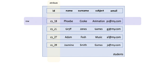
In this diagram there is a table called students; it is being used to hold

information about students attending a meeting. The table has 5 attributes (or

columns) deﬁned for id, name, surname, subject and email.

In this case, the id is probably what is known as a primary key. The primary key

is a property that is used to uniquely identify the student row; it cannot be omitted

and must be unique (within the table). Obviously names and subjects may well be

duplicated as there may be more than one student studying Animation or Games and

students may have the same ﬁrst name or surname. It is probable that the email

column is also unique as students probably don’t share an email address but again

this may not necessarily be the case.

You might at this point wonder why the data in a Relational Database is called

relational and not tables or tabular? The reason is because of a topic known as

relational algebra that underpins Relational Database theory. Relational Algebra

takes its name from the mathematical concept known as a relation. However, for

the purposes of this chapter you don’t need to worry about this and just need to

remember that data is held in tables.

23.2.1 Data Relationships

When the data held in one table has a link or relationship to data held in another

table then an index or key is used to link the values in one table to another. This is

illustrated below for a table of addresses and a table of people who live in that

address. This shows for examp le, that ‘Phoebe Gates’ lives at address ‘addr2’ which

is 12 Queen Street, Bristol, BS42 6YY.

276 23 Introduction to Databases

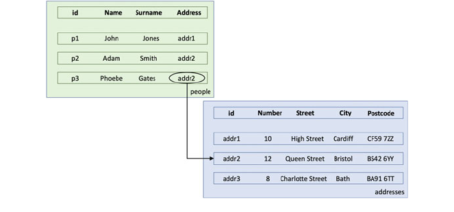
This is an example of a many to one (often written as many:1) relationship; that

is there are many people who can live at one address (in the above Adam Smith also

lives at address ‘addr2’). In Relational Databases there can be several different types

of relationship such as:

• one:one where only one row in one table references one and only one row in

another table. An example of a one to one relationship might be from a person to

an order for a unique piece of jewellery.

• one:many this is the same as the above address example, however in this case

the direction of the relationship is reversed (that is to say that one address in the

addresses table can reference multiple persons in the people table).

• many:many This is where many rows in one table may reference many rows in

a second table. For example, many students may take a particular class and a

student may take many classes. This relationship usually involves an interme-

diate (join) table to hold the associations between the rows.

23.2.2 The Database Schema

The structure of a Relational Database is deﬁned using a Data Deﬁnition Language

or Data Description Language (a DDL).

Typically, the syntax of such a language is limited to the semantics (meaning)

required to deﬁne the structure of the tables. This structure is known as the database

schema. Typically, the DDL has commands such as CREATE TABLE, DROP

TABLE (to delete a table) and ALTER TABLE (to modify the structure of an

existing table).

Many tools provided with a database allow you to deﬁne the structure of the

database without getting too bound up in the syntax of the DDL; however, it is

useful to be aware of it and to understand that the database can be created in this

way. For example, we will use the MySQL database in this chapter. The MySQL

23.2 What Is a Database? 277

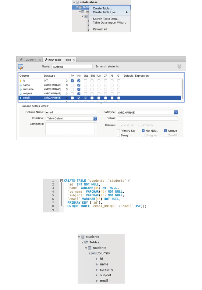
Workbench is a tool that allows you to work with MySQL databases to manage and

query the data held within a particular database instance. For references for mySQL

and the MySQL Workbench see the links at the end of this chapter.

As an example, within the MySQL Workbench we can create a new table using a

menu option on a database:

Using this we can interactively deﬁne the columns that will comprise the table:

Here each column name, its type and whether it is the primary key (PK), not

empty (or Not Null NN) or unique (UQ) have been speci ﬁed. When the changes are

applied, the tool also shows you the DDL that will be used to create the database:

When this is applied a new table is created in the database as shown below:

278 23 Introduction to Databases

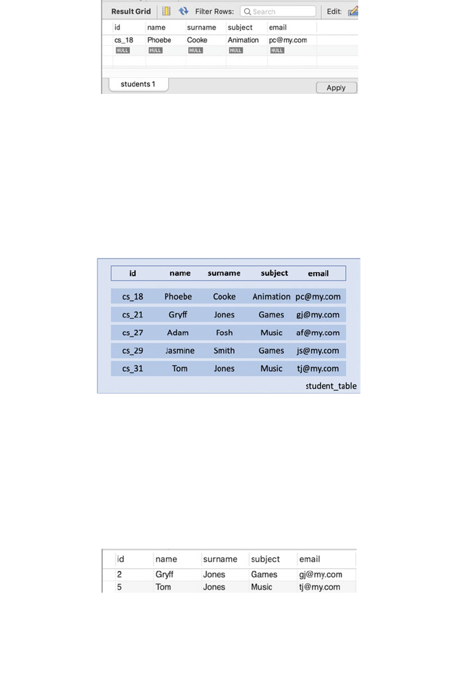
The tool also allows us to populate data into the table; this is done by entering

data into a grid and hitting apply as shown below:

23.3 SQL and Databases

We can now use query languages to identify and return data held in the database

often using speciﬁc criteria.

For example, let us say we want to return all the people who have the surname

Jones from the following table:

We can do this by speci fying that data shoul d be returned where the surname

equals ‘Jones’; in SQL this would look like:

The above SELECT statement states that all the properties (columns or attributes) in

a row in the table students are to be retur ned where the surname equals ‘Jones’. The

result is that two rows are returned:

Note we need to specify the table we are interested in and what data we want to

return (the ‘*’ after the select indicated we want all the data). If we were only

interested in their ﬁrst names then we could use:

SELECT * FROM students where surname='Jones';

SELECT name FROM students where surname='Jones';

23.2 What Is a Database? 279

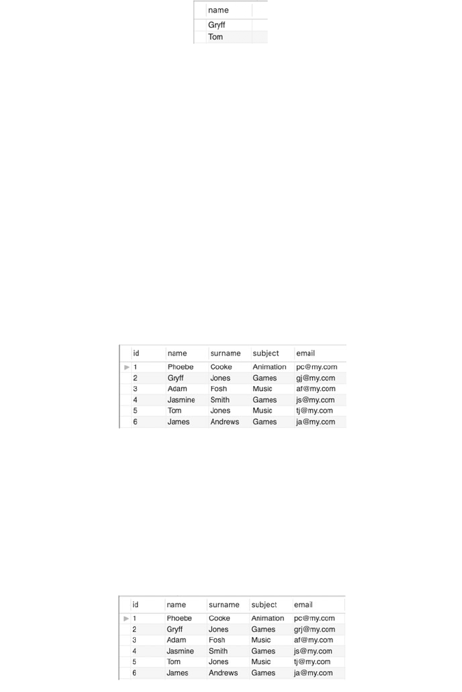
This would return only the names of the students:

23.4 Data Manipulatio n Language

Data can also be inserted into a table or existing data in a table can be updated. This

is done using the Data Manipulation Language (DML).

For example, to insert data into a table we merely need to write an INSERT SQL

statement providing the values to be added and how they map to the columns in the

table:

This would add the row 6 to the table students with the result that the table

would now have an additional row:

Updating an existing row is a little more complicated as it is ﬁrst necessary to

identify the row to be updated and then the data to modify. Thus an UPDATE

statement includes a where clause to ensure the correct row is modiﬁed:

The effect of this code is that the second row in the students table is modiﬁed with

the new email address:

INSERT INTO 'students' ('id', 'name', 'surname', 'subject',

'email') VALUES ('6', 'James', 'Andrews', 'Games',

'[email protected]');

UPDATE 'students' SET 'email'='[email protected]' WHERE 'id'='2';

280 23 Introduction to Databases

23.5 Transactions in Databases

Another important concept within a database is that of a Transaction. A Transaction

represents a unit of work performed within a database management system (or

similar system) against a database instance, and is independent of any other

transaction.

Transactions in a database environment have two main purposes

• To provide a unit of work that allows recovery from failures and keeps a

database consistent even in cases of system failure, when execution stops

(completely or partially). This is because either all the operations within a

transaction are performed or none of them are. Thus, if one operation causes an

error then all the changes being made by the transaction thus far are rolled back

and none of them will have been made.

• To provide isolation between programs accessing a database concurrently. This

means that the work being done by one program will not interact with another

programs work.

A database transaction, by deﬁnition, must be atomic, consistent, isolated

and durable:

• Atomic This indicates that a transaction represents an atomic unit of work; that

is either all the operations in the transaction are performed or none of them are

performed.

• Consistent Once completed the transaction must leave the data in a consistent

state with any data constraints met (such as a row in one table must not reference

an non-existent row in another table in a one to many relationship etc.).

• Isolated This relates to the changes being made by concurrent transactions;

these changes must be isolated from each other. That is, one transaction cannot

see the changes being made by another transaction until the second transaction

completes and all changes are permanently saved into the database.

• Durable This means that once a transaction completes then the changes it has

made are permanently stor ed into the database (until some future transaction

modiﬁes that data).

Database practitioners often refer to these proper ties of database transactions using

the acronym ACID (for Atomic, Consistent, Isolated, Durable).

Not all databases support transactions although all commercial, production

quality databases such as Oracle, Microsoft SQL Server and MySQL, do support

transactions.

23.5 Transactions in Databases 281

23.6 Further Reading

If you want to know more about databases and database management systems here

are some online resources:

•

https://en.wikipedia.org/wiki/Database which is the wikipedia entry for data-

bases and thus acts as a useful quick reference and jumping off point for other

material.

•

https://en.wikibooks.org/wiki/Introduction_to_Computer_Information_Systems/

Database

which provides a short introduction to databases.

•

https://www.techopedia.com/6/28832/enterprise/databases/introduction-to-data-

bases

another useful starting point for delving deeper into databases.

•

https://en.wikipedia.org/wiki/Object_database for information on Object

databases.

•

https://en.wikipedia.org/wiki/NoSQL for an introduction to No SQL or non

relational databases.

•

https://www.mysql.com/ for the MySQL Database.

•

https://dev.mysql.com/downloads/workbench The MySQL Workbench home

page.

•

https://www.mongodb.com/ for the home page of the MongoDB site.

•

http://couchdb.apache.org/ for the Apache Couch Database.

If you want to explore the subject of database design (that is design of the tables and

links between tables in a database) then these references may help:

•

https://en.wikipedia.org/wiki/Database_design the wikipedia entry for database

design.

•

https://www.udemy.com/cwdatabase-design-introduction/ which covers most of

the core ideas within database design.

•

http://en.tekstenuitleg.net/articles/software/database-design-tutorial/intro.html

which provides another tutorial that covers most of the core elements of data-

base design.

If you wish to explore SQL more then see:

•

https://en.wikipedia.org/wiki/SQL the wikipedia site for SQL

•

https://www.w3schools.com/sql/sql_intro.asp which is the W3 school material

on SQL and as such an excellent resource.

•

https://www.codecademy.com/learn/learn-sql which is a codecademy site for

SQL.

282 23 Introduction to Databases

Chapter 24

Python DB-API

24.1 Accessing a Database from Python

The standard for accessing a database in Python is the Python DB-API. This

speciﬁes a set of standard interfaces for modules that wish to allo w Python to access

a speciﬁc database. The standard is described in PEP 249 (

https://www.python.org/

dev/peps/pep-0249

)—a PEP is a Python Enhancement Proposal.

Almost all Python database access modules adhere to this standard. This means

that if you are moving from one database to another, or attempting to port a Python

program from one database to another, then the APIs you encounter should be very

similar (although the SQL processed by different database can also differ). There are

modules available for most common databases such as MySQL, Oracle,

Microsoft SQL Server etc.

24.2 The DB-API

There are several key elements to the DB_API these are:

• The connect function. The connect() function that is used to connect to a

database and returns a Connection Object.

• Connection Objects. Within the DB-API access to a database is achieved

through connection objects. These connection objects provide access to cursor

objects.

• Cursor objects are used to execute SQL statements on the database.

• The result of an execution. These are the results that can be fetched as a

sequence of sequences (such a tuple of tuples). The standard can thus be used to

select, insert or update information in the database.

J. Hunt, Advanced Guide to Python 3 Programming,

Undergraduate Topics in Computer Science,

https://doi.org/10.1007/978-3-030-25943-3_24

283

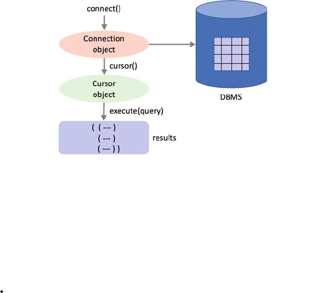
These elements are illustrated below:

The standard speciﬁes a set of functions and objects to be used to connect to a

database. These include the connection function, the Connection Object and the

Cursor object.

The above elements are described in more detail below.

24.2.1 The Connect Function

The connection function is deﬁned as:

connect(parameters...)

It is used to make the initial connection to the database. The connection returns a

Connection Object. The parameters required by the connection function are data-

base dependent.

24.2.2 The Connection Object

The Connection Object is returned by the connect() function. The Connection

object provides several methods including:

• close() used to close the connection once you no longer need it. The con-

nection will be unusable from this point onwards.

• commit() used to commit a pending transaction.

284 24 Python DB-API

• rollback() used to rollback all the changes made to the database since the

last transaction commit (optional as not all databases provide transaction

support).

• cursor() returns a new Cursor object to use with the connection.

24.2.3 The Cursor Object

The Cursor object is returned from the connection.cusor() method.

A Cursor Object represents a database cursor, which is used to manage the context

of a fetch operation or the execution of a database command. Cursors support a

variety of attributes and methods:

• cursor.execu te(operation, parameters) Prepare and execute a

database operation (such as a query statement or an update command).

Parameters may be provided as a sequence or mapping and will be bound to

variables in the operation. Variables are speciﬁed in a database-speciﬁc notation.

• cursor.rowco unt a read-only attribute providing the number of rows that

the last cursor.execute() call returned (for select style statements) or

affected (for update or insert style statements).

• cursor.descr iption a read only attribute providing information on the

columns present in any results returned from a SELECT operation.

• cursor.close () closes the cursor. From this point on the cursor will not be

usable.

In addition, the Cursor object also provides several fetch style methods. These

methods are used to return the results of a database query. The data returned is

made up of a sequence of sequences (such as a tuple of tuples) where each inner

sequence represents a single row returned by the SELECT statement. The fetch

methods deﬁned by the standard are:

• cursor.fetch one() Fetch the next row of a query result set, returning a

single sequence, or None when no more data is available.

• cursor.fetch all() Fetch all (remaining) row s of a query result, returning

them as a sequence of sequences.

• cursor.fetch man(size) Fetch the next set of rows of a query result,

returning a sequence of sequences (e.g. a tuple of tuples). An empty sequence is

returned when no more rows are available. The number of rows to fetch per call

is speciﬁed by the parameter.

24.2 The DB-API 285

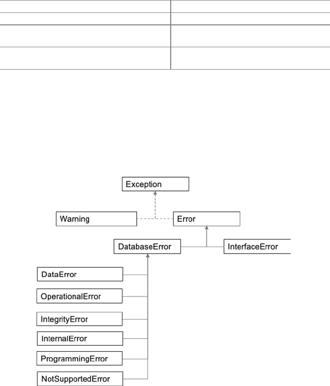
24.2.4 Mappings from Database Types to Python Types

The DB-API standard also speciﬁes a set of mappings from the types used in a

database to the types used in Python. For a full listing see the DB-API standard

itself but the key mappings include:

Date(year, month, day) Represents a database date

Time(hour, minute, second) Represents a time database value

Timestamp(year, month, day, hour,

minute, second)

Holds a database time stamp value

String Used to represent string like database data

(such as VARCHARs)

24.2.5 Generating Errors

The stand ard also speciﬁes a set of Exceptions that can be thrown in different

situations. These are presented below and in the following table:

The above diagram illustrates the inheritance hierarchy for the errors and warning

associated with the standard. Note that the DB-API Warning and Error both

extend the Exception class from standard Python; however, depending on the

speciﬁc implementation there may be one or more additional classes in the hier-

archy between these classes. For example, in the PyMySQL module there is a

286 24 Python DB-API

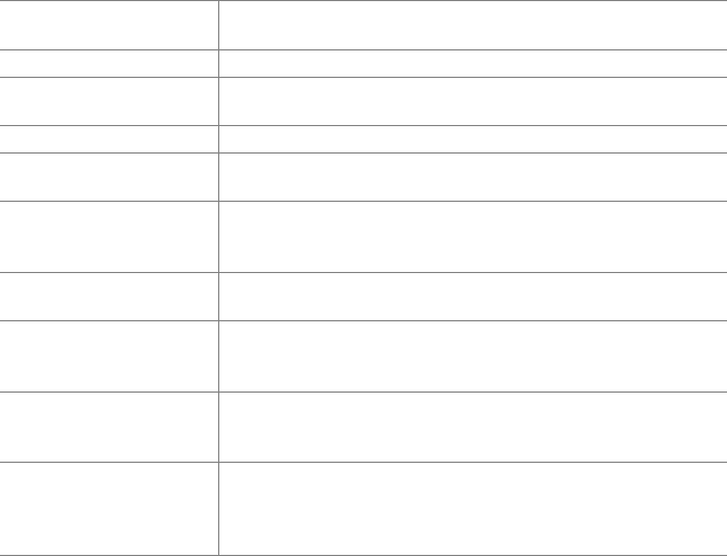
MySQLError class that extends Exception and is then extended by both

Warning and Error.

Also note that Warning and Error have no relationship with each other. This

is because Warnings are not considered Errors and thus have a separate class

hierarchies. However, the Error is the root class for all database Error classes.

A description of each Warning or Error class is provided below.

Warning Used to warn of issues such as data truncations during inserting,

etc.

Error The base class of all other error exceptions

InterfaceError Exception raised for errors that are related to the database

interface rather than the database itself

DatabaseError Exception raised for errors that are related to the database

DataError Exception raised for errors that are due to problems with the data

such as division by zero, numeric value out of range, etc.

OperationalError Exception raised for errors that are related to the database’s

operation and not necessarily under the control of the

programmer, e.g. an unexpected disconnect occurs, etc.

IntegrityError Exception raised when the relational integrity of the database is

affected

InternalError Exception raised when the database encounters an internal error,

e.g. the cursor is not valid anymore, the transaction is out of sync,

etc.

ProgrammingError Exception raised for programming errors, e.g. table not found,

syntax error in the SQL statement, wrong number of parameters

speciﬁed, etc.

NotSupportedError Exception raised in case a method or database API was used

which is not supported by the database, e.g. requesting a

.rollback() on a connection that does not support

transactions or has transactions turned off

24.2.6 Row Descriptions

The Cursor object has an attribute description that provides a sequence of

sequences; each sub sequence provides a description of one of the attributes of the

data returned by a SELECT statement. The sequenc e describing the attribute is

made up of up to seven items, these include:

• name representing the name of the attribute,

• type_code which indicates what Python type this attribute has been mapped

to,

• display_size the size used to display the attribute,

• internal_siz e the size used internally to represent the value,

24.2 The DB-API 287

• precision if a real numeric value the precision supported by the attribute,

• scale indicates the scale of the attribute,

• null_ok this indicates whether null values are acce ptable for this attribute.

The ﬁrst two items (name and type_ code) are mandatory, the other ﬁve are

optional and are set to None if no meaningful values can be provided.

24.3 Transactions in PyMySQL

Transactions are managed in PyMySQL via the database connection object. This

object provides the following method:

• connection.c ommit() this causes the current transaction to commit all the

changes made permanently to the database. A new transaction is then started.

• connection.r ollback() this causes all changes that have been made so

far (but not permanently stored into the database i.e. Not committed) to be

removed. A new transaction is then started.

The standard does not specify how a database interface should manage turning

on and off transaction (not least because not all databases support transactions).

However, MySQL does support transactions and can work in two modes; one

supports the use of transactions as already described; the other uses an auto commit

mode. In auto commit mode each command sent to the database (whether a

SELECT statement or an INSERT/UPDATE statement) is treated as an independent

transaction and any changes are automatically committed at the end of the state-

ment. This auto commit mode can be turned on in PyMySQL using:

• connection.a utocommit(True) turn on autocommit (False to turn off

auto commit which is the default).

Other associated methods include

• connection.g et_autocommit() which returns a boolean indicating

whether auto commit is turned on or not.

• connection.b egin() to explicitly begin a new transaction.

24.4 Online Resources

See the following online resources for more information on the Python Database

API:

288 24 Python DB-API

• https://www.python.org/dev/peps/pep-0249/ Python Database API Speciﬁcation

V2.0.

•

https://wiki.python.org/moin/DatabaseProgramming Database Programming in

Python.

•

https://docs.python-guide.org/scenarios/db/ Databases and Py thon.

24.4 Online Resources 289

Chapter 25

PyMySQL Module

25.1 The PyMySQL Module

The PyMySQL module provides access to a MySQL database from Python. It

implements the Python DB-API v 2.0. This module is a pure Python database

interface implementation meaning that it is portable across different operating

systems; this is notable because some database interface modules are merely

wrappers around other (native) implementations that may or may not be available

on different operating systems. For example, a native Linux based database inter-

face module may not be available for the Windows operating system. If you are

never going to switch between different operating systems, then this is not a

problem of course.

To use the PyMySQL module you will need to install it on your computer. This

will involve using a tool such as Anaconda or adding it to your PyCharm project.

You can also use pip to install it:

pip install PyMySQ

25.2 Working with the PyMySQL Module

To use the PyMySQL module to access a database you will need to follow these

steps.

1. Import the module.

2. Make a co nnection to the host machine running the database and to the database

you are using.

3. Obtain a cursor object from the connection object.

4. Execute some SQL using the cursor.execute() method.

J. Hunt, Advanced Guide to Python 3 Programming,

Undergraduate Topics in Computer Science,

https://doi.org/10.1007/978-3-030-25943-3_25

291

5. Fetch the result(s) of the SQL using the cursor object (e.g. fetchall,

fetchmany or fetchone).

6. Close the database connection.

These steps are essentially boiler plate, code that is you will use them whenever

you access a database via PyMySQL (or indeed any DB-API compliant module).

We will take each of these steps in turn.

25.2.1 Importing the Module

As the PyMySQL module is not one of the built-in modules provided by default

with Python you will need to import the module into your code, for example using

import pymsql

Be careful with the case used here as the module name is pymysql in the code

(if you try to import PyMySQL Python will not ﬁnd it!).

25.2.2 Connect to the Database

Each databa se module will have their own speciﬁcs for connecting to the database

server; these usually involve specifying the machine that the database is running on

(as databases can be quiet resource intensive, they are often run on a separate

physical computer), the user to use for the connection and any security information

required such as a password and the database instance to connect to. In most cases a

database is looked after by a database management system (a DBMS) that can

manage multiple database instances and it is therefore necessary to specify which

database instance you are interested in.

For MySQL, the MySQL database server is a DBMS that can indeed look after

multiple database instances. The pymysql.connect function thus requires the

following information when connecting to the database is:

• The name of the machine hosting the MySQL database server e.g. dbserver.

mydomain.com . If you want to connect to the same machine as your Python

program is running on, then you can use localhost. This is a special name

reserved for the local machine and avoids you needing to worry about the name

of your local computer.

• The user name to use for the connection. Most databases limit access to their

databases to named users. These are not necessary users such as humans that log

into a system but rather entities that are allo wed to connect to the database and

perform certain operations. For example, one user may only be able to read data

in the database where as another user is allowed to insert new data into the

292 25 PyMySQL Module

database. These users are authenticated by requiring them to provide a

password.

• The password for the user.

• The database instance to connect to. As mentioned in the previous chapter a

Database Management System (DMS) can manage multiple database instances

and thus it is necessary to say which database instance you are interested in.

For example:

# Open database connection

connection =

pymysql.connect('localhost','username','password','uni-

database')

In this case the machine we are connecting to is ‘localhost’ (that is the same

machine as the Python program itself is running on), the user is represented by

‘username’ and ‘password’ and the database instance of interest is called

‘uni-database’.

This returns a Connection object as per the DB-API standard.

25.2.3 Obtaining the Cursor Object

You can obtain the cursor object from the connection using the cursor()

method:

# prepare a cursor object using cursor() method

cursor = connection.cursor()

25.2.4 Using the Cursor Object

Once you have obtained the cursor object you can use it to execute an SQL query or

a DML insert, update or delete statement. The following example uses a simple

select statement to select all the attributes in the students table for all rows currently

stored in the students table:

# execute SQL query using execute() method.

cursor.execute('SELECT * FROM students')

Note that this met hod executes the SELECT statement but does not return the set

of results directly. Instead the execute method returns an integer indicating the

number of rows either affected by the modiﬁcation or returned as part of the query.

In the case of a SELECT statement the number retur ned can be used to determine

which type of fetch method to use.

25.2 Working with the PyMySQL Module 293

25.2.5 Obtaining Information About the Results

The Cursor Object can also be used to obtain information about the results to be

fetched such as how many rows there are in the results and what the type is of each

attribute in the results:

• cusor.rowcou nt() this is a read-only property that indicates the number of

rows returned for a SELECT statement or rows affected for a UPDATE or

INSERT statement.

• cursor.descr iption() this is a read-only property that provides a

description of each attribute in the results set. Each description provides the

name of the attribute and an indication of the type (via a type_code) as well

as further information on whether the value can be null or not and for numbers

scale, precision and size information.

An example of using these two properties is given below:

print('cursor.rowcount', cursor.rowcount)

print('cursor.description', cursor.description)

A sample of the output generated by these lines is given below:

cursor.rowcount 6

cursor.description (('id', 3, None, 11, 11, 0, False),

('name', 253, None, 180, 180, 0, False), ('surname', 253,

None, 180, 180, 0, False), ('subject', 253, None, 180, 180,

0, False), ('email', 253, None, 180, 180, 0, False))

25.2.6 Fetching Results

Now that a successful SELECT statement has been run against the database, we can

fetch the results. The results are returned as a tuple of tuples. As mentioned in the

last chapter there are several different fetch options available including fetchone

(), fetchmany(size) and fetchall(). In the following example we use the

fetchall() option as we know that there are only up to six rows that can be

returned.

# Fetch all the rows and then iterate over the data

data = cursor.fetchall()

for row in data:

print('row:', row)

In this case we loop through each tuple within the data collection and print that row

out. However, we could just as easily have extracted the information in the tuple

294 25 PyMySQL Module

into individual elements. These elements could then be used to construct an object

that could then be processed within an application, for example:

for row in data:

id, name, surname, subject, email = row

student = Student(id, name, surname, subject, email)

print(student)

25.2.7 Close the Connection

Once you have ﬁnished with the database connection it should be closed.

# disconnect from server

connection.close()

25.3 Complete PyMySQL Query Example

A complete listing illustrating connecting up to the database, running a SELECT

statement and printing out the results using a Student class is given below:

import pymysql

class Student:

def __init__(self, id, name, surname, subject, email):

self.id = id

self.name = name

self.surname = surname

self.subject = subject

self.email = email

def __str__(self):

return 'Student[' + str(id) + '] ' + name + ' ' +

surname + ' - ' + subject + ' ' + email

# Open database connection

connection = pymysql.connect('localhost',

'user',

'password',

'uni-database')

# prepare a cursor object using cursor() method

cursor = connection.cursor()

25.2 Working with the PyMySQL Module 295

The output from this program, for the database created in the last chapter is

shown here:

cursor.rowcount 6

cursor.description (('id', 3, None, 11, 11, 0, False),

('name', 253, None, 180, 180, 0, False), ('surname', 253,

None, 180, 180, 0, False), ('subject', 253, None, 180, 180,

0, False), ('email', 253, None, 180, 180, 0, False))

Student[1] Phoebe Cooke - Animation [email protected]

Student[2] Gryff Jones - Games [email protected]

Student[3] Adam Fosh - Music [email protected]

Student[4] Jasmine Smith - Games [email protected]

Student[5] Tom Jones - Music [email protected]

Student[6] James Andrews - Games [email protected]

25.4 Inserting Data to the Database

As well as reading data from a database many applications also need to add new

data to the database. This is done via the DML (Data Manipulation Language)

INSERT statement. The process for this is very similar to running a query against

the database using a SELECT statement; that is, you need to make a connection,

obtain a cursor object and execute the statement. The one difference here is that you

do not need to fetch the results.

# execute SQL query using execute() method.

cursor.execute('SELECT * FROM students')

print('cursor.rowcount', cursor.rowcount)

print('cursor.description', cursor.description)

# Fetch all the rows and then iterate over the data

data = cursor.fetchall()

for row in data:

student_id, name, surname, subject, email = row

student = Student(student_id, name, surname, subject,

email)

print(student)

# disconnect from server

connection.close()

296 25 PyMySQL Module

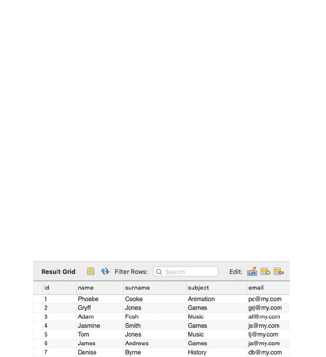
The result of running this code is that the database is updated with a seventh row

for ‘Denise Byrne’. This can be seen in the MySQL Workbench if we look at the

contents of the students table:

There are a couple of points to note about this code example. The ﬁrst is that we

have used the double quotes around the string deﬁning the INSERT command—

this is because a double quotes string allows us to include single quotes within that

string. This is necessary as we need to quote any string values passed to the

database (such as ‘Denise’).

The second thing to note is that by default the PyMySQL database interface

requires the programmer to decide when to commit or rollback a transaction.

A transaction was introduced in the last chapter as an atomic unit of work that must

either be completed or as a whole or rollback so that no changes are made.

However, the way in which we indicate that a transaction is completed is by calling

import pymysql

# Open database connection

connection =

pymysql.connect('localhost', 'user', 'password', 'uni-database')

# prepare a cursor object using cursor() method

cursor = connection.cursor()

try:

# Execute INSERT command

cursor.execute("INSERT INTO students (id, name, surname,

subject, email) VALUES (7, 'Denise', 'Byrne', 'History',

'[email protected]')")

# Commit the changes to the database

connection.commit()

except:

# Something went wrong

# rollback the changes

connection.rollback()

# Close the database connection

connection.close()

25.4 Inserting Data to the Database 297

the commit() method on the database connection. In turn we can indicate that we

want to rollback the current transaction by calling rollback(). In either case,

once the method has been invoked a new transaction is started for any further

database activity.

In the above code we have used a try block to ensure that if everything

succeeds, we will commit the changes made, but if an exception is throw n (of any

kind) we will rollback the transaction—this is a common pattern.

25.5 Updating Data in the Database

If we are able to insert new data into the database, we may also want to update the

data in a database, for example to correct some information. This is done using the

UPDATE statement which must indicate whic h existing row is being updated as

well as what the new data should be.

# Open database connection

connection = pymysql.connect('localhost',

'user',

'password',

'uni-database')

# prepare a cursor object using cursor() method

cursor = connection.cursor()

try:

# Execute UPDATE command

cursor.execute("UPDATE students SET email =

'[email protected]' WHERE id = 7")

# Commit the changes to the database

connection.commit()

except:

# rollback the changes if an exception / error

connection.rollback()

# Close the database connection

connection.close()

import pymysql

In this examp le we are updating the student with id 7 such that their email

address wi ll be changed to ‘[email protected]’. This can be veriﬁed by examining

the contents of the students table in the MySQL Workbench:

298 25 PyMySQL Module

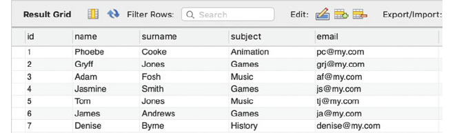
25.6 Deleting Data in the Database

Finally, it is also possible to delete data from a database, for example if a student

leaves their course. This follows the same format as the previous two examples with

the difference that the DELETE statement is used instead:

import pymysql

# Open database connection

connection = pymysql.connect('localhost',

'user',

'password',

'uni-database')

# prepare a cursor object using cursor() method

cursor = connection.cursor()

try:

# Execute DELETE command

cursor.execute("DELETE FROM students WHERE id = 7")

# Commit the changes to the database

connection.commit()

except:

# rollback the changes if an exception / error

connection.rollback()

# Close the database connection

connection.close()

In this case we have deleted the student with id 7. We can see that again in the

MySQL Workbench by examining the contents of the students table after this code

has run:

25.6 Deleting Data in the Database 299

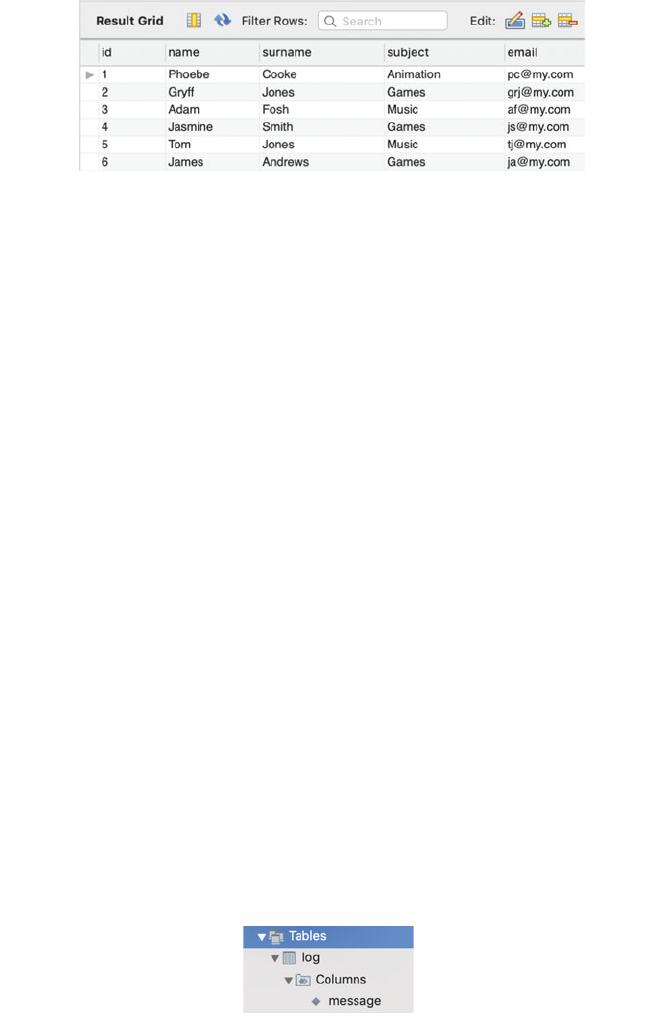
25.7 Creating Tables

It is not just data that you can add to a database; if you wish you can program-

matically create new tables to be used with an application. This process follows

exactly the same pattern as those used for INSERT, UPDATE and DELETE. The

only difference is that the command sent to the databa se contains a CREATE

statement with a description of the table to be created. This is illustrated below:

import pymysql

# Open database connection

connection = pymysql.connect('localhost',

'user',

'password',

'uni-database')

# prepare a cursor object using cursor() method

cursor = connection.cursor()

try:

# Execute CREATE command

cursor.execute("CREATE TABLE log (message VARCHAR(100)

NOT NULL)")

# Commit the changes to the database

connection.commit()

except:

# rollback the changes if an exception / error

connection.rollback()

# Close the database connection

connection.close()

This creates a new table log within the uni-database; this can be seen by looking

at the tables listed for the uni-database within the MySQL Workbench.

300 25 PyMySQL Module

25.8 Online Resources

See the following online resources for more information on the Python Database

API:

•

https://pymysql.readthedocs.io/en/latest/ PyMySQ L Documentation site.

•

https://github.com/PyMySQL/PyMySQL Git hub repository for the PyMySQL

library.

25.9 Exercises

In this exercise you will create a database and tables based on a set of transactions

stored in a current account. You can use the account class you created in the CSV

and Excel chapter for this.

You will need two tables, one for the account information and one for the

transaction history.

The primary key of the account information table can be used as the foreign key

for the transaction history table.

Then write a function that takes an Account object and populates the tables

with the appropriate data.

To create the account information table you might use the following DDL:

Remember to be careful with integers and decimals if you are creating an SQL

string such as:

statement = "INSERT into transactions (idtransactions, type,

amount, account) VALUES (" + str(id) + ", '" + action + "', " +

str(amount) + ", " + str(account_number) + ")"

CREATE TABLE acc_info (idacc_info INT NOT NULL, name

VARCHAR(255) NOT NULL, PRIMARY KEY (idacc_info))

While for the transactions table you might use:

CREATE TABLE transactions (idtransactions INT NOT NULL, type

VARCHAR(45) NOT NULL, amount VARCHAR(45) NOT NULL, account INT

NOT NULL, PRIMARY KEY (idtransactions))"

25.8 Online Resources 301

Part VI

Logging

Chapter 26

Introduction to Logging

26.1 Introduction

Many programming languages have common logging libraries including Java and

C# and of course Python also has a logging module. Indeed the Python loggi ng

module has been part of the built in modules since Python 2.3.

This chapter discusses why you should add logging to your programs, what you

should (and should not) log and why just using the print() function is not

sufﬁcient.

26.2 Why Log?

Logging is typically a key aspect of any production application; this is because it is

important to provide appropriate information to allow futur e investigation following

some event or issue in such applications. These investigations include:

• Diagnosing failures; that is why did an application fail/crash.

• Identifying unusual or unexpected behaviour; which might not cause the

application to fail but which may leave it in an unexpected state or where data

may be corrupted etc.

• Identifying performance or capacity issues; in such situations the application

is performing as expected by it is not meeting some non-functional requirements

associated with the speed at which it is operating or its ability to scale as the

amount of data or the number of users grows.

• Dealing with attempted malicious behaviour in which some outside agent is

attempting to affect the behaviour of the system or to acquire information which

they should not have access to etc. This could happen for example, if you are

creating a Python web application and a user tries to hack into your web server.

J. Hunt, Advanced Guide to Python 3 Programming,

Undergraduate Topics in Computer Science,

https://doi.org/10.1007/978-3-030-25943-3_26

305

• Regulatory or legal compliance. In some cases records of program execution

may be required for regulatory or legal reasons. This is particula rly true of the

ﬁnancial sector where records must be kept for many years in case there is a

need to investigate the organisations’ or individuals’ behaviour.

26.3 What Is the Purpose of Logging?

In general there are therefore two general reason to log what an application is doing

during it operation:

• For diagnostic purposes so that recorded events/steps can be used to analyse the

behaviour of the system when something goes wrong.

• Auditing purposes that allow for later analysis of the behaviour of the system for

business, legal or regulatory purposes. For example, in this case to determine

who did what with what and when.

Without such logged information it is impossible after the event to know what

happened. For example, if all you know is that an application crashed (unexpect-

edly stopped executing) how can you determine what state the application was in,

what functions, methods etc. were being executed and which statements run?

Remember that although a developer may have been using an IDE to run their

applications during development and may possibly been using the debugging

facilities available that allow you to see what functions or methods, statements and

even variable values are place; this is not how most production systems are run. In

general a production Python system will be run either from a command line or

possibly through a short cut (on a Windows box) to simplify running the program.

All the user will know is that something failed or that the behaviour they expected

didn’t occur—if in fact they are aware of any issue at all!

Logs are therefore key to after the event analysis of failures, unexpected beha-

viour or for analysis of the operation of the system for business reasons.

26.4 What Should You Log?

One question that you might be considering at this point is ‘what information

should I log?’.

An application shoul d log enough information so that post event investigators

can unders tand what was happening, when and where. In general this means that

you will want to log the time of the log message, the module/ ﬁlename, function

name or method name executing, potent ially the log level being used (see later) and

in some cases the parameter values/state of the environment, program or class

involved.

306 26 Introduction to Logging

In many cases developers log the entry (and to a lesser extent) the exit from a

function or method. However, it may also be useful to log what happens at branch

points within a function or method so that the logic of the application can be

followed.

All applications should log all errors/exceptions. Although care is needed to

ensure that this is done appropriately. For example if an exception is caught and then

re thrown severa l times it is not necessary to log it every time it is caught. Indeed

doing this can make the log ﬁles much larger, cause confusion when the problem is

being investigated and result in unnecessary overheads. One common approach is to

log an exception where it is ﬁrst raised and caught and not to log it after that.

26.5 What Not to Log

The follow on question to consider is ‘what information should I not log?’.

One general area not to log is any personal or sensitive information including

any information that can be used to identify an individual. This sort of information

is known as PII or Personally Identiﬁcation Information.

Such information includes

• user ids and passwords,

• email addresses,

• data of birth, birth place,

• personally identiﬁable ﬁnancial information such as bank account details, credit

card details etc.,

• biometric information,

• medical/health informat ion,

• government issued personal information such as passport details, drivers license

number, social security numbers, National Insur ance numbers etc.,

• ofﬁcial organisational information such as professional registrations and mem-

bership numbers,

• physical addresses, phone (land-line) numbe rs, mobile phone numbers,

• veriﬁcation elated information such as mother’s maiden name, pets’ names, high

school, ﬁrst school, favourite ﬁlm, etc.,

• it also increasing includes online information relating to social media such as

Facebook or LinkedIn accounts.

All of the above is sensitive information and much of it can be used to identify

an individual; none of this information should be logged directly.

That does not mean that you cannot and shouldn’t log that a user logged in; you

may well need to do that. However, the information should at least be obfuscated

and should not include any information not required. For example you may record

that a user represented by some id attempted to log in at a speci ﬁc time and whether

they were successful or not. However, you should not log their password and may

26.4 What Should You Log? 307

not log the actual userid—instead you may log an id that can be used to map to their

actual userid.

You should also be careful about directly logging data input too an application

directly into a log ﬁle. One way in which a malicious agent can attack an appli-

cation (particularly a web application) is by attempting to send very large amounts

of data to it (as part of a ﬁeld or as a parameter to an operation). If the application

blindly logs all data submitted to it, then the log ﬁles can ﬁll up very quickly. This

can result in the ﬁle store being used by the application ﬁlling up and causing

potential problems for all software using the same ﬁle store. This form of attack is

known as a log (or log ﬁle) injection attack and is wel l documented (see

https://

www.owasp.org/index.php/Log_Injection

which is part of the well respected Open

Web Application Security Project).

Another point to note is that it is not merely enough to log an error. This is not

error handling; logging an error does not mean you have handled it; only that you

have noted it. An application should still decide how it should manage the error or

exception.

In general you should also aim for empty logs in a production syst em; that is

only information that needs to be logged in a production system should be logged

(often information about errors, exceptions or other unexpected behaviour).

However, during testing much more detail is required so that the execution of the

system should be followed. It should therefore be possible to select how much

information is logged depending on the environment the code is running in (that is

within a test environment or within a production environment).

A ﬁnal point to note is that it is important to log information to the correct place.

Many applications (and organisations) log general information to one log ﬁle, errors

and exceptions to another and security information to a third. It is therefore

important to know where your log information is being sent and not to send

information to the wrong log.

26.6 Why Not Just Use Print?

Assuming that you want to log information in your application then next question is

how should you do that? Through this book we have been using the Python print()

function to print out information that indicates results generated by our code but

also at times what is happening with a function or a method etc.

Thus we need to consider whether using the print() function the best way to log

information.

In actual fact, using print() to log information in a production system is almost

never the right answer, this is for several reasons:

• The print() function by default writes strings out to the standard output (stdout)

or standard error output (stderr) which by default directs output to the console/

terminal. For example, when you run an application within an IDE, the output is

308 26 Introduction to Logging

displayed in the Console window. If you run an application from the command

line then the output is directed back to that command/terminal window. Both of

these are ﬁne during development, but what if the program is not run from a

command window, perhaps instead it is started up by the operating system

automatically (as is typical of numerous services such as a print service or a web

server). In this case there is no terminal /console window to send the data to;

instead the data is just lost. As it happens the stdout and stderr output streams

can be directed to a ﬁle (or ﬁles). However, this is typically done when the

program is launched and may be easily omitted. In addition there is only the

option of sending all stdout to a speciﬁc ﬁle or all error output to the stderr.

• Another issue with using the print() function is that all calls to print will be

output. When using most loggers it is possible to specify the log level required.

These different log levels allow different amounts of information to be generated

depending upon the scenario. For example, in a well tested reliable production

system we may only want error related or critical information to be logged. This

will reduce the amount of information we are collecting and reduce any per-

formance impact introduced by logging into the application. However, during

testing phases we may want a far more detailed level of logging.

• In other situations we may wish to change the log level being used for a running

production system without needing to modify the actual code (as this has the

potential to introduced errors into the code). Instead we would like to have the

facility to externally change the way in which the logging system behaves, for

example through a conﬁguration ﬁle. This allows system administrators to

modify the amount and the detail of the information being logged. It typically

also allows the designation of the log information to be changed.

• Finally, when using the print() function a developer can use whatever format

they like, they can include a timestamp on the message or not, they can include

the module or function/method name or not they can include parameters of not.

Using a logging system usually standardises the information generated along

with the log message. Thus all log messages will have (or not have) a times-

tamp, or all messages will include (or not include) information on the function

or method in which they were generated etc.

26.7 Online Resources

For further information on logging see the following:

•

https://en.wikipedia.org/wiki/Log_ﬁle A wikipedia page on logging.

•

https://www.codeproject.com/Articles/42354/The-Art-of-Logging An interest-

ing article on the art of logging.

•

www.owasp.org/index.php The Open Web Application Security Project

(OWASP).

26.6 Why Not Just Use Print? 309

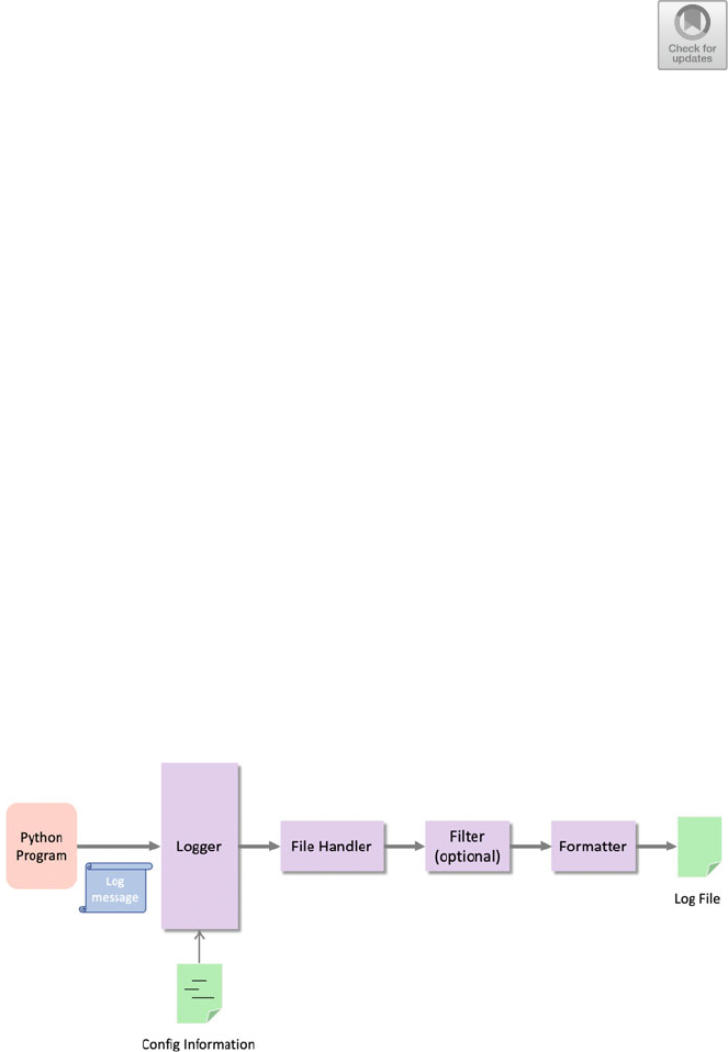
Chapter 27

Logging in Python

27.1 The Logging Module

Python has included a built-in logging module since Python 2.3. This module, the

logging module, deﬁnes functions and classes which implement a ﬂexible log-

ging framework that can be used in any Python application/script or in Python

libraries/modules.

Although different logging frameworks differ in the speciﬁc details of what they

offer; almost all offer the same core elements (although different names are

sometimes used). The Python logging module is no different and the core elements

that make up the logging framework and its processing pipeline are shown below

(note that a very similar diagram could be drawn for logging frameworks in Java,

Scala, C++ etc.).

The following diagram illustrates a Python progra m that uses the built-in Python

logging framework to log messages to a ﬁle.

The core elements of the logging framework (some of which are optional) are

shown above and described below:

J. Hunt, Advanced Guide to Python 3 Programming,

Undergraduate Topics in Computer Science,

https://doi.org/10.1007/978-3-030-25943-3_27

311

• Log Message The is the message to be logged from the application.

• Logger Provides the programmers entry point/interface to the logging system.

The Logger class provides a variety of methods that can be used to log messages

at different levels.

• Handler Handlers determine where to send a log message, default handlers

include ﬁle handlers that send messages to a ﬁle and HTTP handlers that send

messages to a web server.

• Filter This is an optional element in the logging pipeline. They can be used to

further ﬁlter the information to be logged providing ﬁne grained control of

which log messages are actually output (for example to a log ﬁle).

• Formatter These are used to format the log message as required. This may

involve adding timestamps, module and function/method information etc. to the

original log message.

• Conﬁguration Information The logger (and associated handlers, ﬁlters and

formatters) can be conﬁgured either programmatically in Python or through

conﬁguration ﬁles. These conﬁguration ﬁles can be written using key-value

pairs or in a YAML ﬁle (which is a simple mark up language). YAML stand s for

Yet Another Markup Language!

It is worth noting that much of the logging framework is hidden from the

developer who really only sees the logger; the remainder of the logging pipeline is

either conﬁgured by default or via log conﬁguration information typically in the

form of a log conﬁguration ﬁle.

27.2 The Logger

The Logger provides the programmers interface to the logging pipeline.

A Logger object is obtained from the getLogger() function deﬁned in the

logging module. The following code snippet illustrates acquiring the default

logger and using it to log an error message. Note that the logging module must

be imported:

The output from this short application is logged to the console as this is the

default conﬁguration:

This should be used with something unexpected

import logging

logger = logging.getLogger()

logger.error('This should be used with something unexpected'

312 27 Logging in Python

27.3 Controlling the Amount of Information Logged

Log messages are actually associated with a log level. These log levels are intended

to indicate the severity of the message being logged. There are six different log

levels associated with the Python logging framework, these are:

• NOTSET At this level no logging takes place and logging is effectively turned

off.

• DEBUG This level is intended to provide detailed information, typically of

interest when a developer is diagnosing a bug or issues within an application.

• INFO This level is expected to provide less detail than the DEBUG log level as

it is expected to provide information that can be used to conﬁrm that the

application is working as expected.

• WARNING This is used to provide information on an unexpected event or an

indication of some likely problem that a developer or system administration

might wish to investigate further.

• ERROR This is used to provide information on some serious issue or problem

that the application has not been able to deal with and that is likely to mean that

the application cannot function correctly.

• CRITICAL This is the highest level of issue and is reserved for critical situ-

ations such as ones in which the program can no longer continue executing.

The log levels are relative to one another and deﬁned in a hierarchy. Each log

level has a numeric value associated with it as shown below (although you should

never need to use the numbers). Thus INFO is a higher log level than DEBUG,in

turn ERROR is a higher log level than WARNING, INFO, DEBUG etc.

Associated with the log level that a message is logged with, a logger also has a

log level associated with it. The logger will process all mess ages that are at the

loggers log level or above that level. Thus if a logger has a log level of WARNING

then it will log all messages logged using the warning, error and critical

log levels.

Generally speaking, an application will not use the DEBUG level in a production

system. This is usually considered inappropriate as it is only intended for debug

scenarios. The INFO level may be considered appropriate for a production system

although it is likely to produce large amounts of information as it typically traces

the execution of functions and methods. If an application has been well tested and

veriﬁed then it is only really warnings and errors which should occur/be of concern.

It is therefore not uncommon to default to the WARNING level for production

27.3 Controlling the Amount of Information Logged 313

systems (indeed this is why the default log level is set to WARNING within the

Python logging system).

If we now look at the following code that obtains the default logger object and

then uses severa l different logger methods, we can see the effect of the log levels on

the output:

import logging

logger = logging.getLogger()

logger.debug('This is to help with debugging')

logger.info('This is just for information')

logger.warning('This is a warning!')

logger.error('This should be used with something unexpected')

logger.critical('Something serious')

The default log level is set to warning, and thus only messages logged at the

warning level or above will be printed out:

This is a warning!

This should be used with something unexpected

Something serious

As can be seen from this, the messages logged at the debug and info level have been

ignored.

However, the Logger object allows us to change the log level programmatically

using the setLevel() method, for example logger.setLevel(logging.

DEBUG) or via the logging.basicConﬁg(level = logging.DEBUG)

function; both of these will set the logging level to DEBUG. Note that the log level

must be set before the logger is obtained.

If we add one of the above approaches to setting the log level to the previ ous

program we will change the amount of log information generated:

import logging

logging.basicConfig(level=logging.DEBUG)

logger = logging.getLogger()

logger.warning('This is a warning!')

logger.info('This is just for information')

logger.debug('This is to help with debugging')

logger.error('This should be used with something unexpected

logger.critical('Something serious')

314 27 Logging in Python

This will now output all the log messages as debug is the lowest logging level.

We can of course turn off logging by setting the log level to NOTSET

logger.setLevel(logging.NOTSET)

Alternatively you can set the Loggers disabled attribute to True:

logging.Logger.disabled = True

27.4 Logger Methods

The Logger class provides a number of methods that can be used to control what is

logged including:

• setLevel(level ) Sets this logger s log level.

• getEffectiveLevel() Returns this loggers log level.

• isEnabledFor (level) Checks to see if this logger is enabled for the log

level speciﬁed.

• debug(messag e) logs messages at the debug level.

• info(message ) logs messages at the info level.

• warning(mess age) logs messages at the warning level.

• error(messag e) logs messages at the error level.

• critical(mes sage) logs messages at the critical level.

• exception(me ssage) This method logs a message at the error level.

However, it can only be used within an exception handler and includes a stack

trace of any associated exception, for example:

import logging

logger = logging.getLogger()

try:

print('starting')

x = 1 / 0

print(x)

except:

logger.exception('an exception message')

print('Done')

• log(level, message) logs messages at the log level speciﬁed as the ﬁrst

parameter.

27.3 Controlling the Amount of Information Logged 315

In addition there are several methods that are used to manage handlers and

ﬁlters:

• addFilter(ﬁlter) This method adds the speciﬁed ﬁlter ﬁlter to this

logger.

• removeFilter (ﬁlter) The speciﬁed ﬁlter is removed from this logger

object.

• addHandler(h andler) The speciﬁed handler is added to this logger.

• removeHandle r(handler) Removes the speciﬁed handler from this

logger.

27.5 Default Logger

A default (or root) logger is always available from the logging framework.

This logger can be accessed via the functions deﬁned in the logging module.

These functions allow messages to be logged at different levels using methods such

as info(), error(), warning() but without the need to obtain a reference to

a logger object ﬁrst. For example:

import logging

# Set the root logger level

logging.basicConfig(level=logging.DEBUG)

# Use root (default) logger

logging.debug('This is to help with debugging')

logging.info('This is just for information')

logging.warning('This is a warning!')

logging.error('This should be used with something unexpected'

logging.critical('Something serious')

This example sets the logging level for the root or default logger to DEBUG (the

default is WARNING). It then uses the default logger to generate a range of log

messages at different levels (from DEBUG up to CRITICAL). The output from this

program is given below:

DEBUG:root:This is to help with debugging

INFO:root:This is just for information

WARNING:root:This is a warning!

ERROR:root:This should be used with something unexpected

CRITICAL:root:Something serious

Note that the format used by default with the root logger prints the log level, the

name of the logger generating the output and the message. From this you can see

that it is the root longer that is generating the output.

316 27 Logging in Python

27.6 Module Level Loggers

Most modules will not use the root logger to log information, instead they will use a

named or module level logger. Such a logger can be conﬁgured independently of

the root logger. This allows d evelopers to turn on logging just for a module rather

than for a whole application. This can be useful if a developer wishes to investigate

an issue that is located within a single module.

Previous code examples in this chapter have used the getLogger() function

with no parameters to obtain a logger object, for example:

logger = logging.getLogger()

This is really just another way of obtaining a reference to the root logger which

is used by the stand alone logging functions such as logging.info(), log-

ging.debug() function, thus:

logging.warning('my warning')

and

logger.warning('my warning'

Have exactly the same effect; the only difference is that the ﬁrst version involves

less code.

However, it is also possible to create a named logger. This is a separate logger

object that has its own name and can potentially have its own log level, handlers

and formatters etc. To obtain a named logger pass a name string into the

getLogger() method:

logger1 = logging.getLogger('my logger')

This returns a logger object with the name ‘my logger’. Note that this may be a

brand new logger object, however if any other code within the current system has

previously requested a logger called ‘my logger’ then that logger object will be

returned to the current code. Thus multiple calls to getLo gger() with the same

name will always return a reference to the same Logger object.

It is common practice to use the name of the module as the name of the logger;

as only one module with a speciﬁc name should exist within any speciﬁc system.

The name of the module does not need to be hard coded as it can be obtained using

the __name__ module attribute, it is thus common to see:

logger2 = logging.getLogger(__name__)

27.6 Module Level Loggers 317

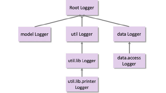
We can see the effect of each of these statements by printing out each logger:

logger = logging.getLogger()

print('Root logger:', logger)

logger1 = logging.getLogger('my logger')

print('Named logger:', logger1)

logger2 = logging.getLogger(__name__)

print('Module logger:', logger2)

When the above code is run the output is:

Root logger: <RootLogger root (WARNING)>

Named logger: <Logger my logger (WARNING)>

Module logger: <Logger __main__ (WARNING)>

This shows that each logger has their own name (the code was run in the main

module and thus the module name was __main__) and all three loggers have an

effective log level of WARNING (which is the default).

27.7 Logger Hierarchy

There is in fact a hierarchy of loggers with the root logger at the top of this hierarchy.

All named loggers are below the root logger.

The name of a logger can actually be a period-separated hierarchic al value such

as util, util.lib and util.lib.printer. Loggers that are further down

the hierarchy are children of loggers further up the logger hierarchy.

For example given a logger called lib, then it will be below the root logger but

above the logger with the name util.lib. This logger will in turn be above the

logger called util.lib.printer. This is illustrated in the following diagram:

318 27 Logging in Python

The logger name hierarchy is analogous to the Python package hierarchy, and

identical to it if you organise your loggers on a per-module basis using the rec-

ommended construction logging.getLogger(__name__).

This hierarchy is important when considering the log level. If a log level has not

been set for the current logger then it will look to its parent to see if that logger has a

log level set. If it does that will be the log level used. This search back up the logger

hierarchy will continue until either an explicit log level is found or the root logger is

encountered which has a default log level of WARNING.

This is useful as it is not necessary to explicitly set the log level for every logger

object used in an application. Instead it is only necessary to set the root log level (or

for a module hierarchy an appropriate point in the module hierarchy). This can then

be overridden where speciﬁcally required.

27.8 Formatters

The are two levels at which you can format the messages logged, these are within

the log message passed to a logging method (such as info() or warn()) and via

the top level conﬁguration that indicates what additional information may be added

to the individual log message.

27.8.1 Formatting Log Messages

The log message can have control characters that indicate what values should be

placed within the message, for example:

logger.warning('%s is set to %d', 'count', 42)

This indicates that the format string expects to be given a string and a number. The

parameters to be substituted into the format string follow the format string as a

comma separated list of values.

27.8.2 Formatting Log Output

The logging pipeline can be conﬁgured to incorporate standard information with

each log message. This can be done globally for all handlers. It is also possible to

programmatically set a speciﬁc formatter on a individual handler; this is discussed

in the next section.

To globally set the output format for log messages use the logging.

basicConﬁg() function using the named parameter format.

27.7 Logger Hierarchy 319

The format parameter takes a string that can contain LogRecord

attributes organised as you see ﬁt. There is a comprehensive list of LogRecord

attributes which can be referenced at

https://docs.python.org/3/library/logging.

html#logrecord-attributes

. The key ones are:

• args a tuple listing the arguments used to call the associated function or

method.

• asctime indicates the time that the log message was created.

• ﬁlename the name of the ﬁle containing the log statement.

• module the module name (the name portion of the ﬁlename).

• funcName the name of the function or method containing the log statement.

• levelname the log level of the log statement.

• message the log message itself as provided to the log method.

The effect of some of these are illustrated below.

import logging

logging.basicConfig(format='%(asctime)s %(message)s',

level=logging.DEBUG)

logger = logging.getLogger(__name__)

def do_something():

logger.debug('This is to help with debugging')

logger.info('This is just for information')

logger.warning('This is a warning!')

logger.error('This should be used with something

nexpected')

logger.critical('Something serious')

do_something()

The above program generates the following log statements:

2019-02-20 16:50:34,084 This is to help with debugging

2019-02-20 16:50:34,084 This is just for information

2019-02-20 16:50:34,085 This is a warning!

2019-02-20 16:50:34,085 This should be used with something

unexpected

2019-02-20 16:50:34,085 Something serious

However, it might be useful to know the log level associated with the log

statements, as well as the function that the log statements were called from. It is

possible to obtain this information by changing the format string passed to the

logging.basicConﬁg() function:

320 27 Logging in Python

Which will now generate the output within log level information and the

function involved:

2019-02-20 16:54:16,250[DEBUG] do_something: This is to help

with debugging

2019-02-20 16:54:16,250[INFO] do_something: This is just for

information

2019-02-20 16:54:16,250[WARNING] do_something: This is a

warning!

2019-02-20 16:54:16,250[ERROR] do_something: This should be

used with something unexpected

2019-02-20 16:54:16,250[CRITICAL] do_something: Something

serious

We can even control the format of the date time information associated with the

log statement using the datafmt parameter of the logging.basicConﬁg()

function:

logging.basicConfig(format='%(asctime)s %(message)s',

datefmt='%m/%d/%Y %I:%M:%S %p', level=logging.DEBUG)

This format string uses the formatting options used by the datetime.strp-

time() function (see

https://docs.python.org/3/library/datetime.html#strftime-

strptime-behavior

) for information on the control characters, in this case

• %m—Month as a zero-padded decimal number e.g. 01, 11, 12.

• %d—Day of the month as a zero-padded decimal number e.g. 01, 12 etc.

• %Y—Year with century as a decimal number e.g. 2020.

• %I—Hour (12-h clock) as a zero-padded decimal number e.g. 01, 10 etc.

• %M—Minute as a zero-padded decimal number e.g. 0, 01, 59 etc.

• %S—Second as a zero-padded decimal number e.g. 00, 01, 59 etc.

• %p—Either AM or PM.

Thus the output generated using the above datefmt string is:

02/20/2019 05:05:18 PM This is to help with debugging

02/20/2019 05:05:18 PM This is just for information

02/20/2019 05:05:18 PM This is a warning!

02/20/2019 05:05:18 PM This should be used with something

unexpected

02/20/2019 05:05:18 PM Something serious

To set a formatter on an individual handler see the next section.

logging.basicConfig(format='%(asctime)s[%(levelname)s]

%(funcName)s: %(message)s', level=logging.DEBUG)

27.8 Formatters 321

27.9 Online Resources

For further information on the Python logging framework see the follow ing:

•

https://docs.python.org/3/library/logging.html The standard library documenta-

tion on the logging facilities in Python.

•

https://docs.python.org/3/howto/logging.html A how to guide on logging from

the Python standard library documentation.

•

https://pymotw.com/3/logging/index.html Python Module of the Week logging

page.

27.10 Exercises

This exercise will involve adding logging to the Account class you have been

working on in this book.

You should add log methods to each of the methods in the class using either the

debug or info methods. You should also obtain a module logger for the account

classes.

322 27 Logging in Python

Chapter 28

Advanced Logging

28.1 Introduction

In this chapter we go further into the conﬁguration and modiﬁcation of the Python

logging module. In particular we will look at Handlers (used to determine the

destination fo log messages), Filters which can be used by Handlers to provide ﬁner

grained control of log output and logger conﬁguration ﬁles. We conclude the

chapter by considering performance issues associated with logging.

28.2 Handlers

Within the logging pipeline, it ia handlers that send the log message to their ﬁnal

destination.

By default the handler is set up to direct output to the console/terminal associ-

ated with the running program. However, this can be changed to send the log

messages to a ﬁle, to an email service, to a web server etc. Or indeed to any

combination of these as there can be multiple handlers conﬁgured for a logger. This

is shown in the diagram below:

J. Hunt, Advanced Guide to Python 3 Programming,

Undergraduate Topics in Computer Science,

https://doi.org/10.1007/978-3-030-25943-3_28

323

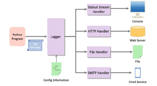
In the above diagram the logger has been conﬁgured to send all log messages to four

different handlers which allow a log message to be written to the console, to a web

server to a ﬁle and to an email service. Such a behaviour may be required because:

• The web server will allow developers access to a web interface that allows them to

see the log ﬁles even if they do not have permission to access a production server .

• The log ﬁle ensures that all the log data is permanently stored in a ﬁle within the

ﬁle store.

• An email message may be sent to a notiﬁcation system so that someone will be

notiﬁed that there is an issue to be investigated.

• The console may still be available to the syst em administrators who may wish to

look at the log messages generated.

The Python logging framework comes with several different handlers as sug-

gested above and listed below:

• logging.Stre am Handler sends messages to outputs such as stdout,

stderr etc.

• logging.FileHandler sends log messages to ﬁles. There are several

varieties of File Handler in addition to the basic FileHandler, these include

the logging.handlers.RotatingFileHandler (which will rotate log

ﬁles based on a maximum ﬁle size) and logging.handlers.

TimeRotating FileHandler (which rotates the log ﬁle at speciﬁed time

intervals e.g. daily).

• logging.hand lers.SocketHandler which sends messages to a TCP/IP

socket where it can be received by a TCP Server.

• logging.hand lers.SMTPHandler that sends messages by the SMT P

(Simple Mail Transfer Protocol) to a email server.

• logging.hand lers.SysLogHandler that sends log messages to a Unix

syslog program.

324 28 Advanced Logging

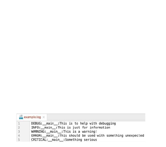
• logging.hand lers.NTEventLogHandler that sends message to a

Windows event log.

• logging.hand lers.HTTPHandler which sends messages to a HTTP

server.

• logging.Null Handler that does nothing with error messages. This is often

used by library developers who want to include logging in their applications but

expect developers to set up an appropriate handler when they use the library.

All of these handlers can be conﬁgured programmatically or via a conﬁguration ﬁle.

28.2.1 Setting the Root Outpu t Handler

The following example, uses the logging.basicConﬁg() function to set up the

root logger to use a FileHandler that will write the log messages to a ﬁle called

‘example.log’:

Note that if no handler is speciﬁed for a named logger then it delegates output to the

parent (in this case the root) logger. The ﬁle generated for the above program is

shown below:

import logging

# Sets a file handler on the root logger to

# save log messages to the example.log file

logging.basicConfig(filename='example.log' ,level=logging.DEBUG)

# If no handler is explicitly set on the name logger

# it will delegate the messages to the parent logger to handle

logger = logging.getLogger(__name__)

logger.debug('This is to help with debugging' )

logger.info('This is just for information' )

logger.warning('This is a warning!' )

logger.error('This should be used with something unexpected' )

logger.critical('Something serious' )

28.2 Handlers 325

As can be seen from this the default formatter is now conﬁgured for a

FileHandler. This FileHandler adds the log message level before the log

message itself.

28.2.2 Programmatically Setting the Handler

It is also possible to programmatically create a handler and set it for the logger. This

is done by instantiating one of the existing handler classes (or by subclassing an

existing handler such as the root Handler class or the FileHander etc.). The

instantiated handler can then be added as a handler to the logger (remember the

logger can have multiple handlers this is why the method is called addHandler

() rather than something such as setHandler).

An example of explicitly setting the FileHandler for a logger is given below:

The result of running this code is that a log ﬁle is created with the logged messages:

import logging

# Empty basic config turns off default console handler

logging.basicConfig()

logger = logging.getLogger(__name__)

logger.setLevel(logging.DEBUG)

# create file handler which logs to the specified fil

file_handler = logging.FileHandler('detailed.log')

# Add the handler to the Logger

logger.addHandler(file_handler)

# 'application' code

def do_something():

logger.debug('debug message')

logger.info('info message')

logger.warning('warn message')

logger.error('error message')

logger.critical('critical message')

logger.info('Starting')

do_something()

logger.info('Done')

326 28 Advanced Logging

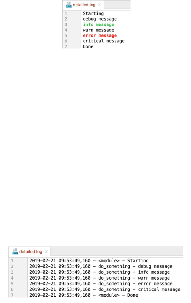
Given that this is a lot more code than using the basicConﬁg() function; the

question here might be ‘Why bother?’. The answer is two fold:

• You can have different handlers for different loggers rather than setting the

handler to be used centrally.

• Each handler can have its own format set so that logging to a ﬁle has a different

format to logging to the console.

We can set the format for the handler by instantiating the logging.

Formatter class with an appropriate format string. The formatter object can then

be applied to a handler using the setFormatter() method on the handler

object.

For example, we can modify the above code to include a formatter that is then

set on the ﬁle handler as shown below.

The log ﬁle now generated is modiﬁed such that each message includes a time stamp,

the function name (or modul e if at the module level) as well as the log message itself.

# create file handler which logs to the specified file

file_handler = logging.FileHandler('detailed.log' )

# Create formatter for the file_handler

formatter = logging.Formatter('%(asctime)s - %(funcName)s -

%(message)s' )

file_handler.setFormatter(formatter)

logger.addHandler(file_handler)

28.2 Handlers 327

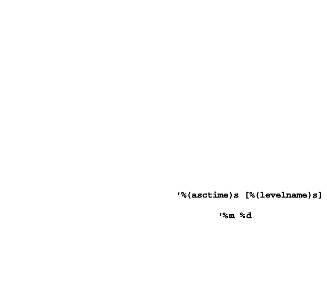
28.2.3 Multiple Handlers

As suggested in the previous section we can create multiple handlers to send log

messages to different locations; for example from the console, to ﬁles and even

email servers. The following program illustrates setting up both a ﬁle handler and a

console handler for a module level logger.

To do this we create two handlers the ﬁle_handler and the con-

sole_handler. As a side effect we can also give them different log levels and

different formatters. In this case the ﬁle_handler inherits the log level of the

logger itself (which is DEBUG) while the console_handler has its log level set

explicitly at WARNING. This means different amounts of information will be logged

to the log ﬁle than the console output.

We have also set different formatters on each handler; in this case the log ﬁle

handler’s formatter provides more information than the console handlers formatter.

Both handlers are then added to the logger before it is used.

# Multiple Handlers and formatters

import logging

# Set up the default root logger to do nothing

logging.basicConfig(handlers=[logging.NullHandler()])

# Obtain the module level logger and set level to DEBUG

logger = logging.getLogger(__name__)

logger.setLevel(logging.DEBUG)

# Create file handler

file_handler = logging.FileHandler('detailed.log')

# Create console handler with a higher log level

console_handler = logging.StreamHandler()

console_handler.setLevel(logging.WARNING)

# Create formatter for the file handler

fh_formatter = logging.Formatter(

%(name)s.%(funcName)s: %(message)s',

datefmt=

- -%Y %I:%M:%S

%p')

file_handler.setFormatter(fh_formatter)

328 28 Advanced Logging

The output from this program is now split between the log ﬁle and the console

out, as shown below:

28.3 Filters

Filters can be used by Handlers to provide ﬁner grained control of the log output.

A ﬁlter can be added to a logger using the logger.addFilter() method.

A Filter can be created by extending the logging.Filter class and

# Create formatter for the console handler

console_formatter = logging.Formatter('%(asctime)s -

%(funcName)s - %(message)s')

console_handler.setFormatter(console_formatter)

# Add the handlers to logger

logger.addHandler(console_handler)

logger.addHandler(file_handler)

# 'application' code

def do_something():

logger.debug('debug message')

logger.info('info message')

logger.warning('warn message')

logger.error('error message')

logger.critical('critical message')

logger.info('Starting')

do_something()

logger.info('Done')

28.2 Handlers 329

implementing the ﬁlter() method. This method takes a log record. This log

record can be validated to determine if the record should be output or not. If it

should be output then True is returned, if the record should be ignored False

should be returned.

In the following example, a ﬁlter called MyFilter is deﬁned that will ﬁlter out

all log messages containing the string ‘John’. It is added as a ﬁlter to the logger and

then two log messages are generated.

The output shows that only the log message that does not contain the string

‘John’ is output:

28.4 Logger Conﬁgurati on

All the examples so far in this chapter have used programmatic conﬁguration of the

logging framework. This is certainly feasible as the examples show, but it does

require a code change if you wish to alter the logging level for any particular logger,

or to change where a particular handler is routing the log messages.

For most production systems a better solution is to use an external conﬁguration

ﬁle which is loaded when the application is run and is used to dynamically con-

ﬁgure the logging framework. This allows system administrators and others to

change the log level, the log destination, the log format etc. without needing to

change the code.

import logging

class MyFilter(logging.Filter):

def filter(self, record):

if 'John' in record.msg:

return False

else:

return True

logging.basicConfig(format='%(asctime)s %(message)s',

level=logging.DEBUG)

logger = logging.getLogger()

logger.addFilter(MyFilter())

logger.debug('This is to help with debugging')

logger.info('This is information on John')

2019-02-20 17:23:22,650 This is to help with debugging

330 28 Advanced Logging

The logging conﬁguration ﬁle can be written using several standard formats from

JSON (the Java Script Object Notation), to YAML (Yet Another Markup Language)

format, or as a set of key-value pairs in a.conf ﬁle. For further information on the

different options available see the Python logging module documentation.

In this book we will brieﬂy explore the YAML ﬁle format used to conﬁgure

loggers.

The above YAML code is stored in a ﬁle called logging.conf.yaml;

however you can call this ﬁle anything that is meaningful.

The YAML ﬁle alw ays starts with a version number. This is an integer value

representing the YAML schema version (currently this can only be the value 1). All

other keys in the ﬁle are optional, they include:

• formatters—this lists one or more formatters; each formatter has a name which

acts as a key and then a format value which is a string deﬁning the format of a

log message.

• ﬁlters—this is a lit of ﬁlter names and a set of ﬁlter deﬁnitions.

• handlers—this is a list of named handlers. Each handler deﬁnition is made up of

a set of key value pairs where the keys deﬁne the class used for the ﬁlter

(mandatory), the log level of the ﬁlter (optional), the formatter to use with the

handler (optional) and a list of ﬁlters to apply (optional).

• loggers—provides one or more named loggers. Each logger can indicate the log

level (optional) and a list of handlers (opti onal). The propagate option can be

used to stop messages propagating to a parent logger (by setting it to False).

• root—this is the conﬁguration for the root logger.

version: 1

formatters:

myformatter:

format: '%(asctime)s [%(levelname)s] %(name)s.%(funcName)s:

%(message)s'

handlers:

console:

class: logging.StreamHandler

level: DEBUG

formatter: myformatter

stream: ext://sys.stdout

loggers:

myLogger:

level: DEBUG

handlers: [console]

propagate: no

root:

level: ERROR

handlers: [console]

28.4 Logger Conﬁguration 331

This ﬁle can be loaded into a Python application using the PyYAML module.

This provides a YAML parser that can load a YAML ﬁle as a dictionary structure

that can be passed to the logging.conﬁg.dictConﬁg() function. As this is a

ﬁle it must be opened and closed to ensure that the resource is handled appropri-

ately; it is therefore best managed using the with-as statement as shown below:

This will open the YAML ﬁle in read-only mode and close it when the two

statements have been executed. This snippet is used in the following application

that loads the logger conﬁguration from the YAML ﬁle:

ith open('logging.config.yaml' , 'r') as f:

config = yaml.safe_load(f.read())

logging.config.dictConfig(config)

import logging

import logging.config

import yaml

ith open('logging.config.yaml', 'r') as f:

config = yaml.safe_load(f.read())

logging.config.dictConfig(config)

logger = logging.getLogger('myLogger')

# 'application' code

def do_something():

logger.debug('debug message')

logger.info('info message')

logger.warning('warn message')

logger.error('error message')

logger.critical('critical message')

logger.info('Starting')

do_something()

logger.info('Done')

332 28 Advanced Logging

The output from this using the earlier YAML ﬁle is:

28.5 Performance Considerations

Performance when logging should always be a consideration. In general you should

aim to avoid performing any unnecessary work when logging is disabled (or dis-

abled for the level being used). This may seem obvious but it can occur in several

unexpected ways.

One example is string concatenation. If a message to be logged involves string

concatenation; then that string concatenation will always be performed when a log

method is being invoked. For example:

This will always result in the string being generated for count and total

before the call is made to the debug function; even if the debug level is not turned

on. However using a format string will avoid this. The formatting involved will

only be performed if the string is to be used in a log message. You should therefore

always use string formatting to populate log messages. For erxmaple:

Another potential optimisation is to use the logger.isEnabledFor

(level) method as a guard against running the log statement. This can be useful

in situations where an associated operation must be performed to support the

logging operation and this operation is expensive. For example:

2019-02-21 16:20:46,466 [INFO] myLogger.<module>: Starting

2019-02-21 16:20:46,466 [DEBUG] myLogger.do_something: debug

essage

2019-02-21 16:20:46,466 [INFO] myLogger.do_something: info

essage

2019-02-21 16:20:46,466 [WARNING] myLogger.do_something: warn

essage

2019-02-21 16:20:46,466 [ERROR] myLogger.do_something: error

essage

2019-02-21 16:20:46,466 [CRITICAL] myLogger.do_something:

critical message

2019-02-21 16:20:46,466 [INFO] myLogger.<module>: Done

logger.debug('Count: ' + count + ', total: ' + total)

logger.debug(' Count: %d, total: %d ', count, 42)

if logger.isEnabledFor(logging.DEBUG):

logger.debug('Message with

%s, %s', expensive_func1(),

expensive_func2())

28.4 Logger Conﬁguration 333

Now the two expensive functions will only be executed if the DEBUG log level

is set.

28.6 Exercises

Using the logging you dded to the Account class int he last chapter, you should load

the log conﬁguration information from a YAML ﬁle similar to that used in this

chapter.

This should be loaded into the application program used to drive the account

classes.

334 28 Advanced Logging

Part VII

Concurrency and Parallelism

Chapter 29

Introduction to Concurrency

and Parallelism

29.1 Introduction

In this chapter we will introduce the concepts of concurrency and parallelism. We

will also brieﬂy consider the related topic of distribution. After this we will consider

process synchronisation, why object oriented approaches are well suited to con-

currency and parallelism before ﬁnishing with a short discussion of threads versus

processes.

29.2 Concurrency

Concurrency is deﬁned by the dictionary as

two or more events or circumstances happening or existing at the same time.

In Computer Science concurrency refers to the ability of different parts or units of a

program, algorithm or problem to be executed at the same time, potentially on

multiple processors or multiple cores.

Here a processor refers to the central processing unit (or CPU) or a computer

while core refers to the idea that a CPU chip can have multiple cores or processors

on it.

Originally a CPU chip had a single core. Tha t is the CPU chip had a single

processing unit on it. However, over time, to increase computer pe rformance,

hardware manufacturers added additional cores or processing units to chips. Thus a

dual-core CPU chip has two processing units while a quad-core CPU chip has four

processing units. This means that as far as the operating system of the computer is

concerned, it has multiple CPUs on which it can run programs.

Running processing at the same time, on multiple CPUs, can substantially

improve the overall performance of an application.

J. Hunt, Advanced Guide to Python 3 Programming,

Undergraduate Topics in Computer Science,

https://doi.org/10.1007/978-3-030-25943-3_29

337

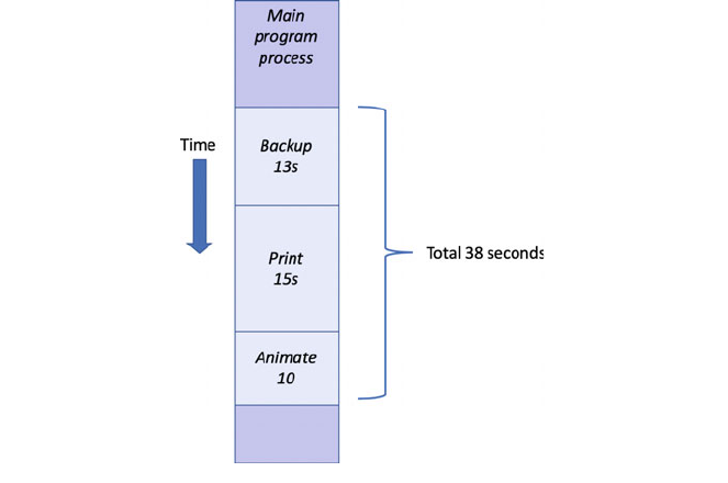
For example, let us assume that we have a program that will call three inde-

pendent functions, these functions are:

• make a backup of the current data held by the program,

• print the data currently held by the program,

• run an animation using the current data.

Let us assume that these functions run sequentially, with the following timing s:

• the backup function takes 13 s,

• the print function takes 15 s,

• the animation function takes 10 s.

This would result in a total of 38 s to perform all three operations. This is illustrated

graphically below:

However, the three functions are all completely independent of each other. That

is they do not rely on each other for any results or behaviour; they do not need one

of the other functions to complete before they can complete etc. Thus we can run

each function concurrently.

If the underlying operating system and program language being used support

multiple proces ses, then we can potentially run each function in a separate process

at the same time and obtain a signiﬁcant speed up in overall execution time.

If the application starts all three functions at the same time, then the maximum

time before the main process can continue will be 15s, as that is the time taken by

the longest function to execute. However, the main program may be able to con-

tinue as soon as all three functions are started as it also does not depend on the

338 29 Introduction to Concurrency and Parallelism

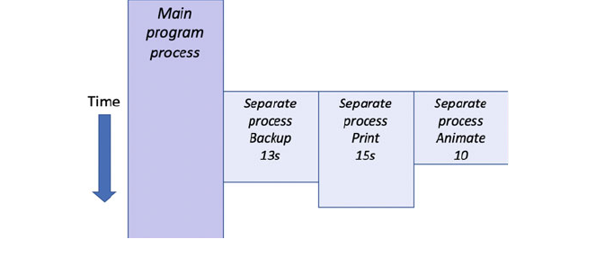
results from any of the functions; thus the delay may be negligible (although there

will typically be some small delay as each process is set up). This is shown

graphically below:

29.3 Parallelism

A distinction its often made in Computer Science between concurrency and

parallelism.

In concurrency, separate independent tasks are performed potentially at the same

time.

In paral lelism, a large complex task is broken down into a set of subtasks. The

subtasks represent part of the overall problem. Each subtask can be executed at the

same time. Typically it is necessary to combine the results of the subtasks together

to generate an overall result. These subtasks are also very similar if not functionally

exactly the same (although in general each subtask invocation will have been

supplied with different data).

Thus parallelism is when multiple copies of the same functionality are run at the

same time, but on different data.

Some examples of where parallelism can be applied include:

• A web search engine. Such a system may look at many, many web pages. Each

time it does so it must send a request to the appropriate web site, receive the

result and process the data obtained. These steps are the same whether it is the

BBC web site, Microsoft’s web site or the web site of Cambridge University.

Thus the requests can be run sequentially or in parallel.

• Image Processing. A large image may be broken down into slices so that each

slice can be analysed in parallel.

29.2 Concurrency 339

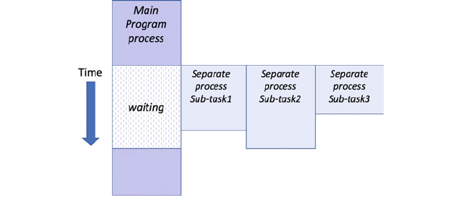
The following diagram illustrates the basic idea behind parallelism; a main program

ﬁres off three subtasks each of which runs in parallel. The main program then waits

for all the subtasks to complete before combining together the results from the

subtasks before it can continue.

29.4 Distribution

When implementing a concurrent or parallel solution, where the resulting processes

run is typically an implementation detail. Conceptually these processes could run

on the same processor, physical machine or on a remote or distributed machine. As

such distribution, in which problems are solved or processes executed by sharing

the work across multiple physical machines, is often related to concurrency and

parallelism.

However, there is no requirement to distribute work across physical machines,

indeed in doing so extra work is usually involved.

To distribute work to a remote machine, data and in many cases code, must be

transferred and made available to the remote machine. This can result in signiﬁcant

delays in running the code remotely and may offset any potent ial pe rformance

advantages of using a physically separate computer. As a result many concurrent/

parallel technologi es default to executing code in a separate process on the same

machine.

29.5 Grid Computing

Grid Computing is based on the use of a network of loosely coupled computers, in

which each computer can have a job submitted to it, which it will run to completion

before returning a result.

340 29 Introduction to Concurrency and Parallelism

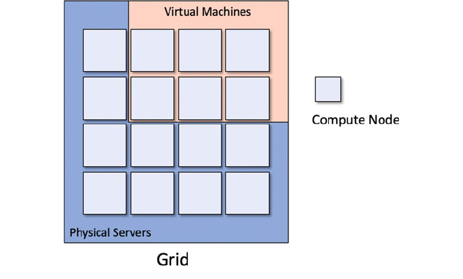
In many cases the grid is made up of a heterogeneous set of computers (rather

than all computers being the same) and may be geographically dispersed. These

computers may be comprised of both physical computers and virtual machines.

A Virtual Machine is a piece of software that emulates a whole computer and

runs on some underlying hardware that is shared with other virtual machines. Each

Virtual Machine thinks it is the only computer on the hardware; however the virtual

machines all share the resources of the physical compu ter. Multiple virtual

machines can thus run simultaneously on the same physical computer. Each virtual

machine provides its own virtual hardware, including CPUs, memory, hard drives,

network interfaces and other devices. The virtual hardware is then mapped to the

real hardware on the physical machine which saves costs by reducing the need for

physical hardware systems along with the associated maintenance costs, as well as

reducing the power and cooling demands of multiple computers .

Within a grid, software is used to manage the grid nodes and to submit jobs to

those nodes. Such software will receive the jobs to perform (programs to run and

information about the environment such as libraries to use) from clients of the grid.

These jobs are typically added to a job queue before a job scheduler submits them

to a node within the grid. When any results are generated by the job they are

collected from the node and returned to the client. This is illustrated below:

29.5 Grid Computing 341

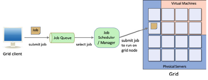
The use of grids can make distributing concurrent/parallel processes amongst a

set of physical and virtual machines much easier.

29.6 Concurrency and Synchronisation

Concurrency relates to executing multiple tasks at the same time. In many cases

these tasks are not related to each other such as printing a document and refreshing

the User Interface. In these cases, the separate tasks are completely independent and

can execute at the same time without any interaction.

In other situations multiple concurrent tasks need to interact; for example, where

one or more tasks produce data and one or more other tasks consume that data. This

is often referred to as a producer-consumer relationship. In other situations, all

parallel processes must have reached the same point before some other behaviour is

executed.

Another situation that can occur is where we want to ensure that only one

concurrent task executes a piece of sensitive code at a time; this code must therefore

be protected from concurrent access.

Concurrent and parallel libraires need to provide facilities that allow for such

synchronisation to occur.

29.7 Object Orientation and Concurrency

The concepts behind object-oriented programming lend themselves particularly

well to the concepts associ ated with concurrency. For example, a system can be

described as a set of discrete objects communicating with one another when nec-

essary. In Python, only one object may execute at any one moment in time within a

single interpreter. However, conceptually at least, there is no reason why this

restriction should be enforced. The basic concepts behind object orientation still

hold, even if each object executes within a separate independent process.

342 29 Introduction to Concurrency and Parallelism

Traditionally a message send is treated like a procedural call, in which the

calling object’s execution is blocked until a response is returned. However, we can

extend this model quite simply to view each object as a concurrently executable

program, with activity starting when the object is created and continuing even when

a message is sent to another object (unless the response is required for further

processing). In this model, there may be very many (concurrent) objects executing

at the same time. Of course, this introduces issues associated with resource allo-

cation, etc. but no more so than in any concurrent system.

One implication of the concurrent object model is that objects are larger than in

the traditional single execution thread approach, because of the overhead of having

each object as a separate thread of execution. Overheads such as the need for a

scheduler to handling these execution threads and resource allocation mechanisms

means that it is not feasible to have integers, characters, etc. as separate processes.

29.8 Threads V Processes

As part of this discussion it is useful to understand what is meant by a process.

A process is an instance of a computer program that is being executed by the

operating system. Any process has three key elements; the program being executed,

the data used by that program (such as the variables used by the program) and the

state of the process (also known as the execution context of the program).

A (Python) Thread is a preemptive lightweight process.

A Thread is considered to be pre-emptive because every thread has a chance to

run as the main thread at some point. When a thread gets to execute then it will

execute until

• completion,

• until it is waiting for some form of I/O (Input/Output),

• sleeps for a period of time,

• it has run for 15 ms (the current threshold in Python 3).

If the thread has not completed when one of the above situations occurs, then it will

give up being the executing thread and another thread will be run instead. This

means that one thread can be interrupted in the middle of performing a series of

related steps.

A thread is a considered a lightweight process because it does not possess its

own address space and it is not treated as a separa te entity by the host operating

system. Instead, it exists within a single machine process using the same address

space.

It is useful to get a clear idea of the difference between a thread (running within a

single machine process) and a multi-process system that uses separate processes on

the underlying hardware.

29.7 Object Orientation and Concurrency 343

29.9 Some Terminology

The world of concurrent programming is full of terminology that you may not be

familiar with. Some of those terms and concepts are outlined below:

• Asynchronous versus Synchronous invocations. Most of the method, function

or procedure invocations you will have seen in programming represent syn-

chronous invocations. A synchronous method or function call is one which

blocks the calling code from executing until it returns. Such calls are typically

within a single thread of execution. Asynchronous calls are ones where the ﬂow

of control immediately returns to the callee and the caller is able to execute in its

own thread of execution. Allowing both the caller and the call to continue

processing.

• Non-Blocking versus Blocking code. Blocking code is a term used to describe

the code running in one thread of execution, waiting for some activity to

complete which causes one of more separate threads of execution to also be

delayed. For example, if one thread is the producer of some data and other

threads are the consumers of that data, then the consumer treads cannot continue

until the producer generates the data for them to consume. In contrast,

non-blocking means that no thread is able to indeﬁnitely delay others.

• Concurrent versus Parallel code. Concurrent code and parallel code are

similar, but different in one signiﬁcant aspect. Concurrency indicates that two or

more activities are both making progress even though they might not be exe-

cuting at the same point in time. This is typically achieved by continuously

swapping competing processes between execution and non-execution. This

process is repeated until at least one of the threads of execution (Threads) has

completed their task. This may occur because two threads are sharing the same

physical processor with each is being given a short time period in which to

progress before the other gets a short time period to progress. The two threads

are said to be sharing the processing time using a technique known as time

slicing. Parallelism on the other hand implies that there are multiple processors

available allowing each thread to execute on their own processor

simultaneously.

29.10 Online Resources

See the following online resources for information on the topics in this chapter:

•

https://en.wikipedia.org/wiki/Concurrency_(computer_science) Wikipedia page

on concurrency.

•

https://en.wikipedia.org/wiki/Virtual_machine Wikipedia page on Virtual

Machines.

344 29 Introduction to Concurrency and Parallelism

• https://en.wikipedia.org/wiki/Parallel_computing Wikipedia page on par-

allelism.

•

http://tutorials.jenkov.com/java-concurrency/concurrency-vs-parallelism.html

Concurrency versus Parallelism tutorial.

•

https://www.redbooks.ibm.com/redbooks/pdfs/sg246778.pdf IBM Red Book on

an Introduction to Grid Computing.

29.10 Online Resources 345

Chapter 30

Threading

30.1 Introduction

Threading is one of the ways in which Python allows you to write programs that

multitask; that is appearing to do more than one thing at a time.

This chapter presents the threadin g module and uses a short example to

illustrate how these features can be used.

30.2 Threads

In Python the Thread class from the threading module represents an activity

that is run in a separate thread of execution within a single process. These threads of

execution are lightweight, pre-emptive execution threads. A thread is lightweight

because it does not possess its own address space and it is not treated as a separate

entity by the host operat ing system; it is not a process. Instead, it exists within a

single machine process using the same address space as other threads.

30.3 Thread States

When a thread object is ﬁrst created it exists, but it is not yet runnable; it must be

started. Once it has been started it is then runnabl e; that is, it is eligible to be

scheduled for execution. It may switch back and forth between running and being

runnable under the control of the scheduler. The scheduler is responsible for

managing multiple threads that all wish to grab some execution time.

A thread object remains runnable or running until its run() method terminates;

at which point it has ﬁnished its execution and it is now dead. All states between

J. Hunt, Advanced Guide to Python 3 Programming,

Undergraduate Topics in Computer Science,

https://doi.org/10.1007/978-3-030-25943-3_30

347

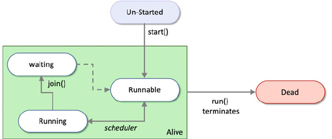
un-started and dead are considered to indicate that the Thread is alive (and therefore

may run at some point). This is shown below:

A Thread may also be in the waiting state; for example, when it is waiting for another

thread to ﬁnish its work before continuing (possibly because it needs the results

produced by that thread to continue). This can be achieved using the join()

method and is also illustrated above. Once the second thread completes the waiting

thread will again become runnable.

The thread which is currently executing is termed the active thread.

There are a few points to note about thread states:

• A thread is considered to be alive unless its run() method terminates after

which it can be considered dead.

• A live thread can be running, runnable, waiting, etc.

• The runnable state indicates that the thread can be execut ed by the processor,

but it is not currently executing. This is because an equal or higher priority

process is already executing, and the thread must wait until the processor

becomes free. Thus the diagram shows that the scheduler can move a thread

between the running and runnable state. In fact, this could happen many times as

the thread executes for a while, is then removed from the processor by the

scheduler and added to the waiting queue, before being returned to the processor

again at a later date.

30.4 Creating a Thread

There are two ways in which to initiate a new thread of execution:

• Pass a reference to a callable object (such as a function or method) into the

Thread class constructor. This reference acts as the target for the Thread to

execute.

348 30 Threading

• Create a subclass of the Thread class and redeﬁne the run() method to

perform the set of actions that the thread is intended to do.

We will look at both approaches.

As a thread is an object, it can be treated just like any other object: it can be sent

messages, it can have instance variables and it can provide methods. Thus, the

multi-threaded aspects of Python all conform to the object-oriented model. This

greatly simpliﬁes the creation of multi-threaded systems as well as the maintain-

ability and clarity of the resulting software.

Once a new instance of a thread is created, it must be started. Before it is started,

it cannot run, although it exists.

30.5 Instantiating the Thread Class

The Thread class can be found in the threading module and therefore must be

imported prior to use. The class Thread deﬁnes a single constructor that takes up

to six optional arguments:

class threading.Thread(group=None,

target=None,

name=None,

args=(),

kwargs={},

daemon=None)

The Thread constructor should always be called using keyword arguments; the

meaning of these arguments is:

• group should be None; reserved for future extension when

a ThreadGroup class is implemented.

• target is the call able object to be invoked by the run() method. Defaults

to None, meaning nothing is called.

• name is the thread name. By default, a unique name is constructed of the form

“Thread-N” where N is an integer.

• args is the argument tuple for the target invocation. Defaults to (). If a single

argument is provided the tuple is not required. If multiple arguments are pro-

vided then each argument is an element within the tuple.

• kwargs is a dictionary of keyword arguments for the target invocation.

Defaults to {}.

• daemon indicates whether this thread runs as a daemon thread or not. If

not None, daemon explicitly sets whether the thread is daemonic. If None (the

default), the daemonic property is inherited from the current thread.

30.4 Creating a Thread 349

Once a Thread is created it must be started to become eligible for execution using

the Thread.start() met hod.

The following illustrates a very simple program that creates a Thread that will

run the simple_worker() function:

from threading import Thread

def simple_worker():

print('hello')

# Create a new thread and start it

# The thread will run the function simple_worker

t1 = Thread(target=simple_worker)

t1.start()

In this example, the threa d t1 will execute the function simple_worker. The

main code will be execut ed by the main thread that is present when the program

starts; there are thus two threads used in the above program; main and t1.

30.6 The Thread Class

The Thread class deﬁnes all the facilities required to create an object that can

execute within its own lightweight process. The key methods are:

• start() Start the thread’s activity. It must be called at most once per thread

object. It arranges for the object’s run() method to be invoke d in a separate

thread of control. This method will raise a RuntimeError if called more than

once on the same thread object.

• run() Method representing the thread’s activity. You may override this

method in a subclass. The standard run() method invokes the callable object

passed to the object’s constructor as the target argument, if any, with positional

and keyword arguments taken from the args and kwargs arguments,

respectively. You should not call this method directly.

• join(timeout = None) Wait until the threa d sent this message terminates.

This blocks the calling thread until the thread whose join()method is called

terminates. When the timeout argument is present and not None, it should be a

ﬂoating-point number specifying a timeout for the operation in seconds (or

fractions thereof). A thread can be join()ed many times.

• name A string used for identiﬁcation purposes only. It has no semantics.

Multiple threa ds may be given the same name. The initial name is set by the

constructor. Giving a thread a name can be useful for debugging purposes.

• ident The ‘thread identiﬁer’ of this thread or None if the thread has not been

started. This is a nonzero integer.

350 30 Threading

• is_alive() Return whether the thread is alive. This method

returns True just before the run() method starts until just after the run()

method terminates. The module function threading.enumerate() re-

turns a list of all alive threads.

• daemon A boolean value indicating whether this thread is a daemon thread

(True) or not (False). This must be set before start() is called, otherwise

a RuntimeError is raised. Its default value is inherited from the creating

thread. The entire Python program exits when no alive non-daemon threads are

left.

An example illustrating using some of these methods is given below:

from threading import Thread

def simple_worker():

print('hello')

t1 = Thread(target=simple_worker)

t1.start()

print(t1.getName())

print(t1.ident)

print(t1.is_alive())

This produces:

hello

Thread-1

123145441955840

True

The join() method can cause one thread to wait for another to complete. For

example, if we want the main thread to wait until a thread completes before it prints

the done message; then we can make it join athatthread:

from threading import Thread

from time import sleep

def worker():

for i in range(0, 10):

print('.', end='', flush=True)

sleep(1)

print('Starting')

# Create read object with reference to worker function

t = Thread(target=worker)

# Start the thread object

30.6 The Thread Class 351

t.start()

# Wait for the thread to complete

t.join()

print('\nDone')

Now the ‘Done’ message should not be printed out until after the worker thread

has ﬁnished as shown below:

Starting

..........

Done

30.7 The Threading Module Functions

There are a set of threading module functions which support working with

threads; these functions include:

• threading.ac tive_count() Return the number of Thread objects cur-

rently alive. The returned count is equal to the length of the list returned

by enumerate().

• threading.cu rrent_thread() Return the current Thread object, cor-

responding to the caller’s thread of control. If the caller’s thread of control was

not created through the threading module, a dummy thread object with

limited functionality is returned.

• threading.ge t_ident() Return the ‘thread identiﬁer’ of the current

thread. This is a nonzero integer. Thread identiﬁers may be recycled when a

thread exits and another thread is created.

• threading.en umerate()Return a list of all Thread objects currently

alive. The list includes daemon threads, dummy thread objects created

by current_thread() and the main thread. It excludes terminated threads

and threads that have not yet been started.

• threading.ma in_thread()Return the main Thread object.

30.8 Passing Arguments to a Thread

Many functions expect to be given a set of parameter values when they are run;

these arguments still need to be passed to the function when they are run via a

separate thread. These parameters can be passed to the function to be executed via

the args parameter, for example:

352 30 Threading

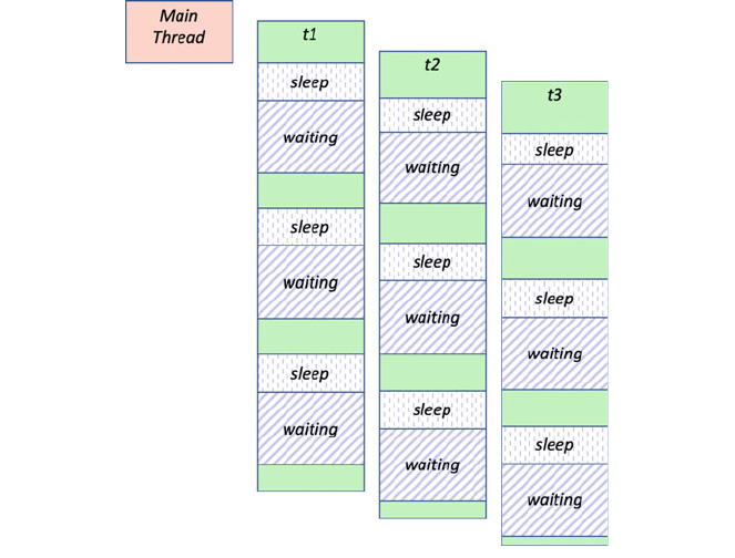
from threading import Thread

from time import sleep

def worker(msg):

for i in range(0, 10):

print(msg, end='', flush=True)

sleep(1)

print('Starting')

t1 = Thread(target=worker, args='A')

t2 = Thread(target=worker, args='B')

t3 = Thread(target=worker, args='C')

t1.start()

t2.start()

t3.start()

print('Done')

In this example, the worker function takes a message to be printed 10 times within

a loop. Inside the loop the thread will print the message and then sleep for a second.

This allows other threads to be execut ed as the Thread must wait for the sleep

timeout to ﬁnish before again becoming runnable.

Three threads t1, t2 and t3 are then created each with a different message. Note

that the worker() function can be reused with each Thread as each invocation

of the function will have its own parameter values passed to it.

The three threads are then started. This means that at this point there is the main

thread, and three worker threads that are Runnable (although only one threa d will

run at a time). The three worker threads each run the worker() function printing

out either the letter A, B or C ten times. This means that once started each thread

will print out a string, sleep for 1 s and then wait until it is selected to run again, this

is illustrated in the following diagram:

30.8 Passing Arguments to a Thread 353

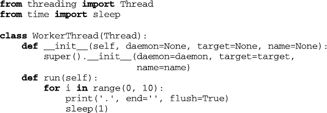
The output generated by this program is illustrated below:

Starting

ABCDone

ABCACBABCABCCBAABCABCABCBAC

Notice that the main thread is ﬁnished after the worker threads have only printed out

a single letter each; however as long as there is at least one non-daemon thread

running the program will not terminate; as none of these threads are marked as a

daemon thread the program continues until the last thread has ﬁnished printing out

the tenth of its letters.

Also notice how each of the threads gets a chance to run on the processor before

it sleeps again; thus we can see the letters A, B and C all mixed in together.

30.9 Extending the Thread Class

The second approach to creating a Thread mentioned earlier was to subclass the

Thread class. To do this you must

1. Deﬁne a new subclass of Thread.

2. Override the run() method.

3. Deﬁne a new __init__() method that calls the parent class __init__()

method to pass the required parameters up to the Thread class constructor.

This is illustrated below where the WorkerThread class passes the name,

target and daemon parameters up to the Thread super class constructor.

Once you have done this you can create an instance of the new WorkerThread

class and then start that instance.

print('Starting')

t = WorkerThread()

t.start()

print('\nDone')

354 30 Threading

The output from this is:

Starting

Done

………

Note that it is common to call any subclasses of the Thread class,

SomethingThread, to make it clear that it is a subclass of the Thread class and

should be treated as if it was a Thread (which of course it is).

30.10 Daemon Threads

A thread can be marked as a daemon thread by setting the daemon property to true

either in the constructor or later via the accessor property.

For example:

from threading import Thread

from time import sleep

def worker(msg):

for i in range(0, 10):

print(msg, end='', flush=True)

sleep(1)

print('Starting')

# Create a daemon thread

d = Thread(daemon=True, target=worker, args='C')

d.start()

sleep(5)

print('Done')

This creat es a background daemon thread that will run the function worker().

Such threads are often used for house keeping tasks (such as background data

backups etc.).

As mentioned above a daemon thread is not enough on its own to keep the

current program from terminating. This means that the daemon thread will keep

looping until the main thread ﬁnishes. As the main thread sleeps for 5 s that allows

the daemon thread to print out about 5 strings before the main thread terminates.

This is illustrated by the output below:

Starting

CCCCCDone

30.9 Extending the Thread Class 355

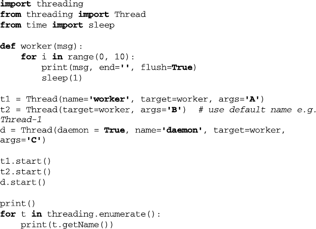
30.11 Naming Threads

Threads can be named; which can be very useful when debugging an application

with multiple threads.

In the following example, three threads have been created; two have been

explicitly given a name related to what they are doing while the middle one has

been left with the default name. We then start all three threads and use the

threading.enumerate() function to loop through all the currently live

threads printing out their names:

The output from this program is given blow:

ABC

MainThread

worker

Thread-1

daemon

ABCBACACBCBACBAABCCBACBACBA

As you can see in addition to the worker thread and the daemo n thread there is a

MainThread (that initiates the whole program) and Thread-1 which is the

thread referenced by the variable t2 and uses the default thread name.

356 30 Threading

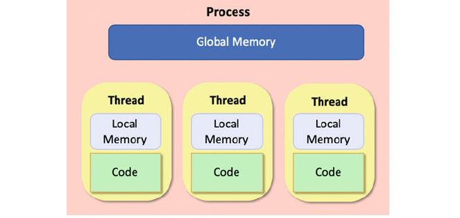
30.12 Thread Local Data

In some situations each Thread requires its own copy of the data it is working

with; this means that the shared (heap) memory is difﬁcult to use as it is inherently

shared between all threads.

To overcome this Python provides a concept known as Thread-Local data.

Thread-local data is data whose values are associated with a thread rather than

with the shared memory. This idea is illustrated below:

To create thread-loc al data it is only necessary to create an instance of threading.

local (or a subclass of this) and store attributes into it. The instances will be thread

speciﬁc; meaning that one thread will not see the values stored by another thread.

For example:

from threading import Thread, local, currentThread

from random import randint

def show_value(data):

try:

val = data.value

except AttributeError:

print(currentThread().name, ' - No value yet')

else:

print(currentThread().name, ' - value =', val)

def worker(data):

show_value(data)

data.value = randint(1, 100)

show_value(data)

print(currentThread().name, ' - Starting')

local_data = local()

show_value(local_data)

30.12 Thread Local Data 357

for i in range(2):

t = Thread(name='W' + str(i),

target=worker, args=[local_data])

t.start()

show_value(local_data)

print(currentThread().name, ' - Done')

The output from this is

MainThread - Starting

MainThread - No value yet

W0 - No value yet

W0 - value = 20

W1 - No value yet

W1 - value = 90

MainThread - No value yet

MainThread - Done

The example presented above deﬁnes two functions.

• The ﬁrst function attempts to access a value in the thread local data object. If the

value is not present an exception is raised (AttributeError). The

show_value() function catches the exception or successfully processes the

data.

• The worker function calls show_value() twice, once before it sets a value in

the local data object and once after. As this function will be run by separate

threads the currentThread name is printed by the show_value()

function.

The main function crates a local data object using the local() function from the

threading library. It then calls show_value() itself. Next it creates two threads to

execute the worker function in passing the local_data object into them; each

thread is then started. Finally, it calls show_value() again.

As can be seen from the output one thread cannot see the data set by another

thread in the local_data object (even when the attribute name is the same).

30.13 Timers

The Timer class represents an action (or task) to run after a certain amount of time

has elapsed. The Timer class is a subclass of Thread and as such also functions

as an example of creating custom threads.

358 30 Threading

Timers are started, as with threads, by calling their start() method. The timer

can be stopped (before its action has begun) by calling the cancel() method. The

interval the timer will wait before executing its action may not be exactly the same

as the interval speciﬁed by the user as another thread may be running when the

timer wishes to start.

The signature of the Timer class constructor is:

Timer(interval, function, args = None, kwargs = None)

An example of using the Timer class is given below:

from threading import Timer

def hello():

print('hello')

print('Starting')

t = Timer(5, hello)

t.start()

print('Done')

In this case the Timer will run the hello function after an initial delay of 5 s.

30.14 The Global Interpreter Lock

The Global Interpreter Lock (or the GIL) is a global lock within the underlying

CPython interpreter that was designed to avoid potential deadlocks between mul-

tiple tasks. It is designed to protect access to Python objects by preventing multiple

threads from executing at the same time.

For the most part you do not need to worry about the GIL as it is at a lower level

than the programs you will be writing.

However, it is worth noting that the GIL is controversial because it prevents

multithreaded Python programs from taking full advantage of multiprocessor sys-

tems in certain situations.

This is because in order to execute a thread must obtain the GIL and only one

thread at a time can hold the GIL (that is the lock it represents). This means that

Python acts like a single CPU machine; only one thing can run at a time. A Thread

will only give up the GIL if it sleeps, has to wait for something (such as some I/O)

30.13 Timers 359

or it has held the GIL for a certain amount of time. If the maximum time that a

thread can hold the GIL has been met the scheduler will release the GIL from that

thread (resulting it stopping execution and now having to wait until it has the GIL

returned to it) and will select another thread to gain the GIL and start to execute.

It is thus impossible for standard Python threads to take advantage of the

multiple CPUs typically available on modern compu ter hardware.

One solution to this is to use the Python multiprocessing library described

in the next chapter.

30.15 Online Resources

See the following online resources for information on the topics in this chapter:

•

https://docs.python.org/3/library/threading.html The Python stand ard Library

documentation on Threading.

•

https://pymotw.com/3/threading/ The Python Module of the Week page on

Threading.

•

https://pythonprogramming.net/threading-tutorial-python/ Tutorial on Python’s

Threading module.

30.16 Exercise

Create a function called printer() that takes a message and a maximum value to

use for a period to sleep.

Within the function create a loop that iterates 10 times. Within the loop

• generate a random number from 0 to the max period speciﬁed and then sleep for

that period of time. You can use the random.randint() funct ion for this.

• Once the sleep period has ﬁnished print out the message passed into the

function.

• Then loop again until this has been repeated 10 times.

Now create ﬁve threads to run ﬁve invocations of the function you produced above

and start all ﬁve threads. Each thread should have a different max_sleep time.

An example program to run the printer function ﬁve times via a set of Threads is

given below:

t1 = Thread(target=printer, args=('A', 10))

t2 = Thread(target=printer, args=('B', 5))

t3 = Thread(target=printer, args=('C', 15))

t4 = Thread(target=printer, args=('D', 7))

t5 = Thread(target=printer, args=('E', 2))

t1.start()

360 30 Threading

t2.start()

t3.start()

t4.start()

t5.start()

An example of the sort of output this could generate is given below:

BAEAEABEDAEAEBEDCECBEEEADCDBBDABCADBBDABADCDCDCCCC

30.16 Exercise 361

Chapter 31

Multiprocessing

31.1 Introduction

The multiprocessing library supports the generation of separate (operating

system level) processes to execute behaviour (such as functions or methods) using

an API that is similar to the Threading API presented in the last chapter.

It can be used to avoid the limitation introduced by the Global Interpreter Lock

(the GIL) by using separate operat ing system processes rathe r than lightw eight

threads (which run within a single process).

This means that the multiprocessing library allows developers to fully

exploit the multiple processor environment of modern computer hardware which

typically has multiple processor cores allowing multiple operations/behaviours to

run in parallel; this can be very signiﬁcant for data analytics, image processing,

animation and games applications.

The multiprocessing library also introduces some new features, most notably the

Pool object for parallelising execution of a callable object (e.g. functions and

methods) that has no equivalent within the Threading API.

31.2 The Process Class

The Process class is the multiprocessing library’s equivalent to the

Thread class in the threading library. It can be used to run a callable object

such as a function in a separate process. To do this it is necessary to create a new

instance of the Process class and then call the start() method on it. Methods

such as join() are also available so that one process can wait for another process

to complete before continuing etc.

The main difference is that when a new Process is created it runs within a

separate process on the underlying operating systems (such as Window, Linux or

J. Hunt, Advanced Guide to Python 3 Programming,

Undergraduate Topics in Computer Science,

https://doi.org/10.1007/978-3-030-25943-3_31

363

Mac OS). In contrast a Thread runs within the same process as the original

program. This means that the process is managed and executed directly by the

operating system on one of the processors that are part of the underlying computer

hardware.

The up side of this is that you are able to exploit the underlying parallelism

inherent in the physical computer hardware. The downside is that a Process takes

more work to set up than the lighter weight Threads.

The constructor for the Process class provides the same set of arguments as

the Thread class, namely:

class multiprocessing.Process(group=None,

target=None,

name=None,

args=(),

kwargs={},

daemon=None)

• group should always be None; it exists solely for compatibility with the

Threading API.

• target is the callable object to be invoked by the run() method. It defaults

to None, meaning nothing is called.

• name is the process name.

• args is the argument tuple for the target invocation.

• kwargs is a dictionary of keyword arguments for the target invocation.

• daemon argument sets the process daemon ﬂag to True or False.

If None (the default), this ﬂag will be inherited from the creating process.

As with the Thread class, the Process constructor should always be called

using keyword arguments.

The Process class also provides a similar set of methods to the Thread class

• start() Start the process’s activity. This must be called at most once per

process object . It arranges for the object’s run() method to be invoked in a

separate process.

• join([timeou t]) If the optional argument timeout is None (the default),

the method blocks until the join ed process terminates. If timeout is a positive

number, it blocks at most timeout seconds. Note that the method

returns None if its process terminates or if the method times out.

364 31 Multiprocessing

• is_alive() Return whether the process is alive. Roughly, a process object is

alive from the moment the start() method returns until the child process

terminates.

The process class also has several attributes:

• name The process’s name. The name is a string used for identiﬁcation purposes

only. It has no semantics. Multiple processes may be given the same name. It

can be useful for debugging purposes.

• daemon The process’s daemon ﬂag, a boolean value. This must be set

before start() is called. The default value is inherited from the creating

process. When a process exits, it attempts to terminate all of its daemonic child

processes. Note that a daemonic process is not allowed to creat e child processes.

• pid Return the process ID. Before the process is spawned, this will be None.

• exitcode The process exit code. This will be None if the process has not yet

terminated. A negative value -N indica tes that the child was terminated by

signal N.

In addition to these methods and attributes, the Process class also deﬁnes

additional process related methods including:

• terminate() Terminate the process.

• kill() Same as terminate() except that on Unix the SIGKILL signal is

used instead of the SIGTERM signal.

• close() Close the Process object, releasing all resources associated with

it. ValueError is raised if the underlying process is still running.

Once close() returns successfully, most of the other methods and attributes

of the Process object will raise a ValueError.

31.3 Working with the Process Class

The following simple program creates three Process objects; each runs the

function worker(), with the string arguments A, B and C respectively. These

three process objects are then started using the start() method.

31.2 The Process Class 365

It is essentially the same as the equivalent program for threads but with the

Process class being used instead of the Thread class.

The output from this application is given below:

Starting

Done

ABCABCABCABCABCABCABCACBACBACB

The main difference between the Thread and Proce ss versions is that the

Process version runs the worker function in separate processes whereas in the

Thread version all the Threads share the same process.

31.4 Alternative Ways to Start a Process

When the start() method is called on a Process, three different approaches to

starting the underlying process are available. These approaches can be set using the

multiprocessing.set_start_method() which takes a string indicating

the approach to use. The actual process initiation mechanisms available depend on

the underlying operating system:

• ‘spawn’ The parent process starts a fresh Python interpreter process. The child

process will only inherit those resources necessary to run the process objects

run() method. In particular, unnecessary ﬁle descriptors and handles from the

from multiprocessing import Process

from time import sleep

def worker(msg):

for i in range(0, 10):

print(msg, end='', flush=True)

sleep(1)

print('Starting')

t2 = Process(target=worker, args='A')

t3 = Process(target=worker, args='B')

t4 = Process(target=worker, args='C')

t2.start()

t3.start()

t4.start()

print('Done')

366 31 Multiprocessing

parent process will not be inherited. Starting a process using this method is

rather slow compared to using fork or forkserver. Available on Unix and

Windows. This is the default on Windows.

• ‘fork’ The parent process uses os.fork() to fork the Python interpreter.

The child process, when it begins, is effectively identical to the parent process.

All resources of the parent are inherited by the child process. Available only on

Unix type operating systems. This is the default on Unix, Linux and Mac OS.

• ‘forkserver’ In this case a server process is started. From then on, whenever

a new process is needed, the parent process connects to the server and requests

that it fork a new process. The fork server process is single threaded so it is safe

for it to use os.fork(). No unnecessary resources are inherited. Available on

Unix style platforms which support passing ﬁle descriptors over Unix pipes.

The set_start_method() should be used to set the start method (and this

should only be set once within a program).

This is illustrated below, where the spawn start method is speciﬁed:

from multiprocessing import Process

from multiprocessing import set_start_method

from time import sleep

import os

def worker(msg):

print('module name:', __name__)

print('parent process:', os.getppid())

print('process id:', os.getpid())

for i in range(0, 10):

print(msg, end='', flush=True)

sleep(1)

def main():

print('Starting')

print('Root application process id:', os.getpid())

set_start_method('spawn')

t = Process(target=worker, args='A')

t.start()

print('Done')

if __name__ == '__main__':

main()

The output from this is shown below:

Starting

Root application process id: 6281

Done

31.4 Alternative Ways to Start a Process 367

module name: __main__

parent process: 6281

process id: 6283

AAAAAAAAAA

Note that the parent process and current process ids are printed out for the worker

() function, while the main() method prints out only its own id. This shows that

the main application process id is the same as the worker process parents’ id.

Alternatively, it is possible to use the get_context() method to obtain a

context object. Context objects have the same API as the multiprocessing

module and allow you to use multiple start methods in the same program, for

example:

ctx = multiprocessing.get_context(‘spawn’)

q = ctx.Queue()

p = ctx.Process(target = foo, args = (q,))

31.5 Using a Pool

Creating Processes is expensive in terms of computer resources. It would therefore

be useful to be able to reuse processes within an application. The Pool class

provides such reusable processes.

The Pool class represents a pool of worker processes that can be used to

perform a set of concurrent, parallel operations. The Pool provides methods which

allow tasks to be ofﬂoaded to these worker processes.

The Pool class provides a constructor which takes a number of arguments:

class multiprocessing.pool.Pool(processes,

initializer, initargs,

maxtasksperchild,

context)

These represent:

• processes is the number of worker processes to use. If proc-

esses is None then the number returned by os.cpu_cou nt() is used.

• initializer If initializer is not None then each worker process will

call initializer(*initargs) when it starts.

• maxtasksperc hild is the number of tasks a worker process can complete

before it will exit and be replaced with a fresh worker process, to enable unused

resources to be freed. The default maxtasksperchild is None, which

means worker processes will live as long as the pool.

368 31 Multiprocessing

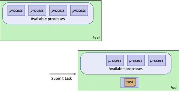
• context can be used to speci fy the context used for starting the worker

processes. Usually a pool is created using the function multiprocessing.

Pool(). Alternatively the pool can be created using the Pool() method of a

context object.

The Pool class provides a range of methods that can be used to submit work to the

worker processes managed by the pool. Note that the methods of the Pool object

should only be called by the process which created the pool.

The following diagram illustrates the effect of submitting some work or task to

the pool. From the list of available proces ses, one process is selected and the task is

passed to the process. The proces s will then execute the task. On completion any

results are returned and the process is returned to the available list. If when a task is

submitted to the pool there are no available processes then the task will be added to

a wait queue until such time as a process is available to handle the task.

The simplest of the methods provided by the Pool for work submission is the map

method:

pool.map(func, iterable, chunksize=None)

This method returns a list of the results obtained by executing the function in

parallel against each of the items in the iterable parameter.

• The func parameter is the callable object to be executed (such as a function or

a method).

• The iteratable is used to pass in any parameters to the function.

• This method chops the iterable into a number of chunks which it submits to the

process pool as separate tasks. The (approximate) size of these chunks can be

speciﬁed by setting chunksize to a positive integer. The method blocks until

the result is ready.

31.5 Using a Pool 369

The following sample program illustrates the basic use of the Pool and the map()

method.

from multiprocessing import Pool

def worker(x):

print('In worker with: ', x)

return x * x

def main():

with Pool(processes=4) as pool:

print(pool.map(worker, [0, 1, 2, 3, 4, 5]))

if __name__ == '__main__':

main()

Note that the Pool object must be closed once you have ﬁnished with it; we are

therefore using the ‘with as’ statement described earlier in this book to handle the

Pool resource cleanly (it will ensure the Pool is closed when the block of code

within the with as statement is completed).

The output from this program is

In worker with: 0

In worker with: 1

In worker with: 2

In worker with: 3

In worker with: 4

In worker with: 5

[0, 1, 4, 9, 16, 25]

As can be seen from this output the map() function is used to run six different

instances of the worker() function with the values provided by the list of inte-

gers. Each instance is executed by a worker process managed by the Pool.

However, note that the Pool only has 4 worker processes, this means that the

last two instances of the worker function must wait until two of the worker

Processes have ﬁnished the work they are doing and can be reused. This can act as a

way of throttling, or controlling, how much work is done in parallel.

A variant on the map() method is the imap_unordered() method. This

method also applies a given function to an iterable but does not attempt to maintain

the order of the results. The results are accessible via the iterable returned by the

function. This may improve the performance of the resulting program.

The following program modiﬁed the worker() function to return its result

rather than print it. These results are then accessible by iterating over them as they

are produced via a for loop:

370 31 Multiprocessing

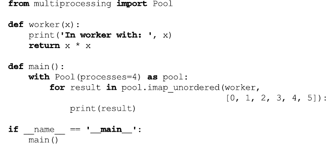
As the new method obtains results as soon as they are available, the order in which

the results are returned may be different, as shown below:

In worker with: 0

In worker with: 1

In worker with: 3

In worker with: 2

In worker with: 4

In worker with: 5

A further method available on the Pool class is the Pool.apply_async()

method. This method allows operations/functions to be executed asynchronously

allowing the method calls to return immediately. That is as soon as the method call

is made, control is returned to the calling code which can continue immediately.

Any results to be collected from the asynchronous operations can be obtained either

by providing a callback function or by using the blocking get() method to obtain

a result.

Two examples are shown below, the ﬁrst uses the blocking get() method. This

method will wait until a result is available before continuing. The second approach

uses a callback function. The callback function is called when a result is available;

the result is passed into the function.

31.5 Using a Pool 371

The output from this is:

In worker with: 6

Result from async: 36

In worker with: 4

In collect_results: 16

31.6 Exchanging Data Between Processes

In some situations it is necessary for two processes to exchange data. However, the

two process objects do not share memory as they are running in separate operating

system level processes. To get around this the multiprocessing library provides the

Pipe() function.

The Pipe() function returns a pair of connection.Connection objects

connected by a pipe which by default is duplex (two-way).

The two connect ion objects returned by Pipe() represent the two ends of the

pipe. Each connection object has send() and recv() methods (among others).

This allows one process to send data via the send() method of one end of the

connection object. In turn a second process can receive that data via the receive

() method of the other connection object. This is illustrated below:

from multiprocessing import Pool

def collect_results(result):

print('In collect_results: ', result)

def worker(x):

print('In worker with: ', x)

return x * x

def main():

with Pool(processes=2) as pool:

# get based example

res = pool.apply_async(worker, [6])

print('Result from async: ', res.get(timeout=1))

with Pool(processes=2) as pool:

# callback based example

pool.apply_async(worker, args=[4],

callback=collect_results)

if __name__ == '__main__':

main()

372 31 Multiprocessing

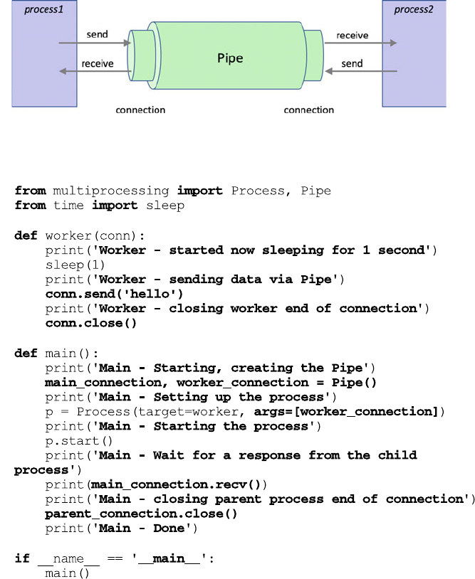
Once a program has ﬁnished with a connection is should be closed using close

().

The following program illustrates how pipe connections are used:

The output from this Pipe example is:

Main - Starting, creating the Pipe

Main - Setting up the process

Main - Starting the process

Main - Wait for a response from the child process

Worker - started now sleeping for 1 second

Worker - sending data via Pipe

Worker - closing worker end of connection

hello

31.6 Exchanging Data Between Processes 373

Main - closing parent process end of connection

Main - Done

Note that data in a pipe may become corrupted if two processes try to read from or

write to the same end of the pipe at the same time. However, there is no risk of

corruption from processes using different ends of the pipe at the same time.

31.7 Sharing State Between Processes

In general, if it can be avoided, then you should not share state between separate

processes. However, if it is unavoidable then the mutiprocessing library

provides two ways in which state (data) can be shared, these are Shared Memory (as

supported by multiprocessing.Value and multiprocessing.Array)

and Server Process.

31.7.1 Process Shared Memory

Data can be stored in a shared memory map using a multiprocessing.Value

or multiprocessing.Array. This data can be accessed by multiple processes.

The constructor for the multiprocessing.Value type is:

multiprocessing.Value

(typecode_or_type, *args, lock = True)

Where:

• typecode_or_ type determines the type of the returned object: it is either a

ctypes type or a one character typecode. For example, ‘d’ indicates a double

precision ﬂoat and ‘i’ indicates a signed integer.

• *args is passed on to the constructor for the type.

• lock If lock is True (the default) then a new recursive lock object is created

to synchronise access to the value. If lock is False then access to the returned

object will not be automatically protected by a lock, so it will not necessarily be

process-safe.

The constructor for multiprocessing.Array is

multiprocessing.Array

multiprocessing.Array(typecode_or_type,

size_or_initializer,

lock=True)

374 31 Multiprocessing

Where:

• typecode_or_type determines the type of the elements of the returned

array.

• size_or_init ializer If size_or_initializer is an integer, then it determi-

nes the length of the array, and the array will be initially zeroed.

Otherwise, size_or_initializer is a sequence which is used to initialise the array

and whose length determines the length of the array.

• If lock is True (the default) then a new lock object is created to synchronise

access to the value. If lock is False then access to the returned object will not

be automatically protected by a lock, so it will not necessarily be “process-safe”.

An example using both the Value and Array type is given below:

from multiprocessing import Process, Value, Array

def worker(n, a):

n.value = 3.1415927

for i in range(len(a)):

a[i] = -a[i]

def main():

print('Starting')

num = Value('d', 0.0)

arr = Array('i', range(10))

p = Process(target=worker, args=(num, arr))

p.start()

p.join()

print(num.value)

print(*arr)

print('Done')

if __name__ == '__main__':

main()

31.8 Online Resources

See the following online resources for information on multiprocessing:

•

https://docs.python.org/3/library/multiprocessing.html The Python standard

Library documentation on MultiProcessing.

•

https://pymotw.com/3/multiprocessing The Python Module of the Week page on

MultiProcessing.

•

https://pythonprogramming.net/multiprocessing-python-intermediate-python-

tutorial

Tutorial on Python’s MultiProcessing module.

31.7 Sharing State Between Processes 375

31.9 Exercises

Write a program that can ﬁnd the factorial of any given number. For example, ﬁnd

the factorial of the number 5 (often written as 5!) which is 1*2*3*4*5and

equals 120.

The factorial is not deﬁned for negative numbers and the factorial of Zero is 1;

that is 0! = 1.

Next modify the program to run multiple factorial calculations in parallel.

Collect all the results together in a list and print that list out.

You an use whichever approach you like to running multiple processes although

a Pool could be a good approach to use.

Your program should compute the factorials of 5, 8, 10, 15, 3, 6, and 4 in

parallel.

376 31 Multiprocessing

Chapter 32

Inter Thread/Process Synchronisation

32.1 Introduction

In this chapter we will look at several facilities supported by both the threading

and multiprocessing libraries that allow for synchronisation and cooperation

between Threads or Processes.

In the remainder of this chapter we will look at some of the ways in which

Python supports synchronisation between multiple Threads and Processes. Note

that most of the libraries are mirrored between threading and multiprocessing so

that the same basic ideas hold for both approaches with, in the main, very similar

APIs. However, you should not mix and match threads and processes. If you are

using Threads then you should only use facilities from the threading library.

In turn if you are using Processes than you should only use facilities in the

multiprocessing library. The examples given in this chapter will use one or

other of the technologies but are relevant for both approaches.

32.2 Using a Barrier

Using a threading.Barrier (or multiprocessing.Barrier) is one of

the simplest ways in which the execution of a set of Threads (or Processes) can be

synchronised.

The threads or processes involved in the barrier are known as the parties that are

taking part in the barrier.

Each of the parties in the barrier can work independently until it reaches the

barrier point in the code.

The barrier represents an end point that all parties must reach before any further

behaviour can be triggered. At the point that all the parties reach the barrier it is

possible to optionally trigger a post-phase action (also known as the barrier call-

back). This post-phase action represents some behaviour that should be run when

J. Hunt, Advanced Guide to Python 3 Programming,

Undergraduate Topics in Computer Science,

https://doi.org/10.1007/978-3-030-25943-3_32

377

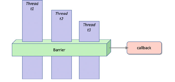
all parties reach the barrier but before allowing those parties to continue. The

post-phase action (the callback) executes in a single thread (or process). Once it is

completed then all the parties are unblocked and may continue.

This is illustrated in the following diagram. Threads t1, t2 and t3 are all involved

in the barrier. When thread t1 reaches the barrier it must wait until it is released by

the barrier. Similarly when t2 reaches the barrier it must wait. When t3 ﬁnally

reaches the barrier the callback is invoked. Once the callback has completed the

barrier releases all three threads which are then able to continue.

An example of using a Barrier object is given below. Note that the function

being invoked in each Thread must also cooperate in using the barrier as the code

will run up to the barrier.wait() method and then wait until all other threads

have also reached this point before being allowed to continue.

The Barrier is a class that can be used to create a barrier object. When the

Barrier class is instantiated, it can be provided with three parameters:

where

• parties the number of individual parties that will participate in the Barrier.

• action is a callable object (such as a function) which, when supplied, will be

called after all the parties have entered the barrier and just prior to releasing

them all.

• timeout If a ‘timeout’ is provided, it is used as the default for all subsequent

wait() calls on the barrier.

Thus, in the following code

b = Barrier(3, action=callback)

Indicates that there will be three parties involved in the Barrier and that the

callback function will be invoked when all three reach the barrier (however the

timeout is left as the default value None).

The Barrier object is created outside of the Threads (or Processes) but must

be made available to the function being executed by the Thread (or Process).

The easiest way to handle this is to pass the barrier into the function as one of the

378 32 Inter Thread/Process Synchronisation

parameters; this means that the function can be used with different barrier objects

depending upon the context.

An example using the Barrier class with a set of Threads is given below:

from threading import Barrier, Thread

from time import sleep

from random import randint

def print_it(msg, barrier):

print('print_it for:', msg)

for i in range(0, 10):

print(msg, end='', flush=True)

sleep(1)

sleep(randint(1, 6))

print('Wait for barrier with:', msg)

barrier.wait()

print('Returning from print_it:', msg)

def callback():

print('Callback Executing')

print('Main - Starting')

b = Barrier(3, callback)

t1 = Thread(target=print_it, args=('A', b))

t2 = Thread(target=print_it, args=('B', b))

t3 = Thread(target=print_it, args=('C', b))

t1.start()

t2.start()

t3.start()

print('Main - Done')

The output from this is:

Main - Starting

print_it for: A

print_it for: B

print_it for: C

ABC

Main - Done

ABCACBACBABCACBCABACBACBBAC

Wait for barrier with: B

Wait for barrier with: A

Wait for barrier with: C

Callback Executing

Returning from print_it: A

Returning from print_it: B

Returning from print_it: C

From this you can see that the print_it() function is run three times con-

currently; all three invocations reach the barrier.wait() statement but in a

different order to that in which they were started. Once the three have reached this

point the callback function is executed before the print_it() function

invocations can proceed.

32.2 Using a Barrier 379

The Barrier class itself provides several methods used to manage or ﬁnd out

information about the barrier:

Method Description

wait(timeout=None) Wait until all threads have notiﬁed the barrier (unless timeout is

reached)—returns the number of threads that passed the barrier

reset() Return barrier to default state

abort() Put the barrier into a broken state

parties Return the number of threads required to pass the barrier

n_waiting Number of threads currently waiting

A Barrier object can be reused any number of times for the same number of

Threads.

The above example could easily be changed to run using Process by altering

the import statement and creating a set of Processes instead of Threads:

from multiprocessing import Barrier, Process

...

print('Main - Starting')

b = Barrier(3, callback)

t1 = Process(target=print_it, args=('A', b))

Note that you should only use threads with a threading.Barrier. In turn

you should only use Processes with a multiprocessing.Barrier.

32.3 Event Signalling

Although the point of using multiple Threads or Processes is to execute separate

operations concurrently, there are times when it is important to be able to allow two

or more Threads or Processes to cooperate on the timing of their behaviour. The

Barrier object presented above is a relatively high-level way to do this; however,

in some cases ﬁner grained control is requi red. The threa ding.Event or

multiprocessing.Event classes can be used for this purpose.

An Event manages an internal ﬂag that callers can either set() or clear().

Other threads can wait() for the ﬂag to be set(), effectively blocking their own

progress until allowed to continue by the Event. The internal ﬂag is initially set to

False which ensures that if a task gets to the Event before it is set then it must wait.

You can infact invoke wait with an optional timeout. If you do not include the

optional timeout then wait() will wait forever while wait(timeout) will wait

up to the timeout given in seconds. If the time out is reached, then the wait

method returns False; otherwise wait returns True.

As an example, the following diagram ill ustrates two processes sharing an event

object. The ﬁrst process runs a function that waits for the event to be set. In turn the

second process runs a function that will set the event and thus release the waiting

process.

380 32 Inter Thread/Process Synchronisation

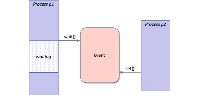
The following program implements the above scenario:

from multiprocessing import Process, Event

from time import sleep

def wait_for_event(event):

print('wait_for_event - Entered and waiting')

event_is_set = event.wait()

print('wait_for_event - Event is set: ', event_is_set)

def set_event(event):

print('set_event - Entered but about to sleep')

sleep(5)

print('set_event - Waking up and setting event')

event.set()

print('set_event - Event set')

print('Starting')

# Create the event object

event = Event()

# Start a Process to wait for the event notification

p1 = Process(target=wait_for_event, args=[event])

p1.start()

# Set up a process to set the event

p2 = Process(target=set_event, args=[event])

p2.start()

# Wait for the first process to complete

p1.join()

print('Done')

32.3 Event Signalling 381

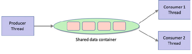
The output from this program is:

Starting

wait_for_event - Entered and waiting

set_event - Entered but about to sleep

set_event - Waking up and setting event

set_event - Event set

wait_for_event - Event is set: True

Done

To change this to use Threads we would merely need to change the import and to

create two Threads:

from threading import Thread, Event

...

print('Starting')

event = Event()

t1 = Thread(target=wait_for_event, args=[event])

t1.start()

t2 = Thread(target=set_event, args=[event])

t2.start()

t1.join()

print('Done')

32.4 Synchronising Concurrent Code

It is not uncommon to need to ensure that critical regions of code are protected from

concurrent execution by multiple Threads or Processes. These blocks of code

typically involve the modiﬁcation of, or access to, shared data. It is therefore

necessary to ensure that only one Thread or Process is updating a shared object at a

time and that consumer threads or processes are blocked while this update is

occurring.

This situation is most common where one or more Threads or Processes are the

producers of data and one or more other Threads or Processes are the consumers of

that data.

This is illustrated in the following diagram.

382 32 Inter Thread/Process Synchronisation

In this diagram the Producer is running in its own Thread (although it could

also run in a separa te Process) and places data onto some common shared data

container. Subsequently a number of independent Consumers can consume that

data when it is available and when they are free to process the data. However, there

is no point in the consumers repeatedly checking the container for data as that

would be a waste of resources (for example in terms of executing code on a

processor and of context switching between multiple Threads or Processes).

We therefore need some form of notiﬁcation or synchronisation between the

Producer and the Consumer to manage this situation.

Python provides several classes in the threading (and also in the multi-

processing) libr ary that can be used to manage critical code blocks. These

classes include Lock, Condition and Semaphore.

32.5 Python Locks

The Lock class deﬁned (both in the threading and the multiprocessing

libraries) provides a mechanism for synchronising access to a block of code. The

Lock object can be in one of two states locked and unlocked (with the initial state

being unlocked). The Lock grants access to a single thread at a time; other threads

must wait for the Lock to become free before progressing.

The Lock class provides two basic methods for acquiring the lock (acquire())

and releasing (release()) the lock.

• When the state of the Lock object is unlocked, then acquire() changes the

state to locked and returns immediately.

• When the state is locked, acquire() blocks until a call to release() in

another thread changes it to unlocked, then the acquire() call resets it to

locked and returns.

• The release() method should only be called in the locked state; it changes

the state to unlocked and returns immediately. If an attempt is made to release an

unlocked lock, a RuntimeError will be raised.

An example of using a Lock object is shown below:

32.4 Synchronising Concurrent Code 383

from threading import Thread, Lock

class SharedData(object):

def __init__(self):

self.value = 0

self.lock = Lock()

def read_value(self):

try:

print('read_value Acquiring Lock')

self.lock.acquire()

return self.value

finally:

print('read_value releasing Lock')

self.lock.release()

def change_value(self):

print('change_value acquiring lock')

with self.lock:

self.value = self.value + 1

print('change_value lock released')

The SharedData class presented above uses locks to control access to critical

blocks of code, speciﬁcally to the read_value() and the change_value()

methods. The Lock object is held internally to the ShareData object and both

methods attempt to acquire the lock before performing their behavior but must then

release the lock after use.

The read_value() method does this explicitly using try: ﬁnally: blocks

while the change_value() method uses a with statement (as the Lock type

supports the Context Manager Protocol). Both approaches achieve the same result

but the with statement style is more concise.

The SharedData class is used below with two simple functions. In this case

the SharedData object has been deﬁned as a global variable but it could also

have been passed into the reader() and updater() functions as an argument.

Both the reader and updater functions loop, attempting to call the read_value()

and change_value() methods on the shared_data object.

As both methods use a lock to control access to the methods, only one thread can

gain access to the locked area at a time. This means that the reader() function

may start to read data before the updater() function has changed the data (or

vice versa).

This is indi cated by the output where the reader thread accesses the value ‘0’

twice before the updater records the value ‘1’. However, the updater() function

runs a second time before the reader gains access to locked block of code which is

why the value 2 is missed. Depending upon the appli cation this may or may not be

an issue.

384 32 Inter Thread/Process Synchronisation

shared_data = SharedData()

def reader():

while True:

print(shared_data.read_value())

def updater():

while True:

shared_data.change_value()

print('Starting')

t1 = Thread(target=reader)

t2 = Thread(target=updater)

t1.start()

t2.start()

print('Done')

The output from this is:

Starting

read_value Acquiring Lock

read_value releasing Lock

read_value Acquiring Lock

read_value releasing Lock

Done

change_value acquiring lock

change_value lock released

change_value acquiring lock

change_value lock released

change_value acquiring lock

change_value lock released

change_value acquiring lock

change_value lock released

Lock objects can only be acquired once; if a thread attempts to acquire a lock on

the same Lock object more than once then a RuntimeError is thrown.

If it is necessary to re-acquire a lock on a Lock object then the threading.

RLock class shoul d be used. This is a Re-entrant Lock and allows the same

Thread (or Process) to acquire a lock multiple times. The code must however

release the lock as many times as it has acquired it.

32.5 Python Locks 385

32.6 Python Conditions

Conditions can be used to synchronise the interaction between two or more Threads

or Processes. Conditions objects support the concept of a notiﬁcation model ; ideal

for a shared data resource being accessed by multiple consumers and producers.

A Condition can be used to notify one or all of the waiting Threads or

Processes that they can proceed (for example to read data from a shared resource).

The methods available that support this are:

• notify() notiﬁes one waiting thread whic h can then continue

• notify_all() notiﬁes all waiting threads that they can continue

• wait() causes a thread to wait until it has been notiﬁed that it can continue

A Condition is always associated with an internal lock which must be

acquired and released before the wait() and notify() methods can be called.

The Condition supports the Context Manager Protocol and can therefore be

used via a with statement (which is the most typical way to use a Condition)to

obtain this lock. For example, to obtain the condition lock and call the wait method

we might write:

ith condition:

condition.wait()

print('Now we can proceed')

The condition object is used in the following example to illustrate how a producer

thread and two consumer threads can cooperate. A DataResource class has been

deﬁned which will hold an item of data that will be shared between a consumer and a

set of producers. It also (internally) deﬁnes a Condition attribute. Note that this

means that the Condition is completely internalised to the DataResource class;

external code does not need to know, or be concerned with, the Condition and its

use. Instead external code can merely call the consumer() and producer()

functions in separate Threads as required.

The consumer() method uses a with statement to obtain the (internal) lock

on the Condition object before waiting to be notiﬁed that the data is available. In

turn the producer() method also uses a with statement to obtain a lock on the

condition object before generating the data attribute value and then notifying

anything waiting on the condition that they can proceed. Note that although the

consumer method obtains a lock on the condition object; if it has to wait it will

release the lock and re obtain the lock once it is notiﬁed that it can continue. This is

a subtly that is often missed.

386 32 Inter Thread/Process Synchronisation

from threading import Thread, Condition, currentThread

from time import sleep

from random import randint

class DataResource:

def __init__(self):

print('DataResource - Initialising the empty data')

self.data = None

print('DataResource - Setting up the Condition object')

self.condition = Condition()

def consumer(self):

"""wait for the condition and use the resource"""

print('DataResource - Starting consumer method in',

currentThread().name)

with self.condition:

self.condition.wait()

print('DataResource - Resource is available to',

currentThread().name)

print('DataResource - Data read in',

currentThread().name, ':', self.data)

def producer(self):

"""set up the resource to be used by the consumer"""

print('DataResource - Starting producer method')

with self.condition:

print('DataResource - Producer setting data')

self.data = randint(1, 100)

print('DataResource - Producer notifying all

aiting threads')

self.condition.notifyAll()

print('Main - Starting')

print('Main - Creating the DataResource object')

resource = DataResource()

print('Main - Create the Consumer Threads')

c1 = Thread(target=resource.consumer)

c1.name = 'Consumer1'

c2 = Thread(target=resource.consumer)

c2.name = 'Consumer2'

print('Main - Create the Producer Thread')

p = Thread(target=resource.producer)

print('Main - Starting consumer threads')

c1.start()

c2.start()

sleep(1)

print('Main - Starting producer thread')

p.start()

print('Main - Done')

32.6 Python Conditions 387

The output from an example run of this program is:

Main - Starting

Main - Creating the DataResource object

DataResource - Initialising the empty data

DataResource - Setting up the Condition object

Main - Create the Consumer Threads

Main - Create the Producer Thread

Main - Starting consumer threads

DataResource - Starting consumer method in Consumer1

DataResource - Starting consumer method in Consumer2

Main - Starting producer thread

DataResource - Starting producer method

DataResource - Producer setting data

Main - Done

DataResource - Producer notifying all waiting threads

DataResource - Resource is available to Consumer1

DataResource - Data read in Consumer1 : 36

DataResource - Resource is available to Consumer2

DataResource - Data read in Consumer2 : 36

32.7 Python Semaphores

The Python Semaphore class implements Dijkstra’s counting semaphore model.

In general, a semaphore is like an integer variable, its value is intended to

represent a number of available resources of some kind. There are typically two

operations available on a semaphore; these operations are acquire() and re-

lease() (although in some libraries Dijkstra’s original names of p() and v()

are used, these operation names are based on the original Dutch phrases).

• The acquire() operation subtracts one from the value of the semaphore,

unless the value is 0, in which case it blocks the calling thread until the

semaphore’s value increases above 0 again.

• The signal() operation adds one to the value, indicating a new instance of

the resource has been added to the pool.

Both the threading.Semaphore and the multiprocessing.Semaphore

classes also supports the Context Manageme nt Proto col.

An optional parameter used with the Semaphore constructor gives the initial

value for the internal counter; it defaults to 1. If the value given is less than 0,

ValueError is raised.

The following example illustrates 5 different Threads all running the same

worker() function. The worker() function attempts to acquire a semaphore; if

it does then it continues into the with statement block; if it doesn’t, it waits until it

can acquire it. As the semaphore is initialised to 2 there can only be two threads that

can acquire the Semaphore at a time.

388 32 Inter Thread/Process Synchronisation

The sample program however, starts up ﬁve threads, this therefore means that the

ﬁrst 2 running Threads will acquire the semaphore and the remaining thee will have

to wait to acquire the semaphore. Once the ﬁrst two release the semaphore a further

two can acquire it and so on.

from threading import Thread, Semaphore, currentThread

from time import sleep

def worker(semaphore):

with semaphore:

print(currentThread().getName() + " - entered")

sleep(0.5)

print(currentThread().getName() + " - exiting")

print('MainThread - Starting')

semaphore = Semaphore(2)

for i in range(0, 5):

thread = Thread(name='T' + str(i),

target=worker,

args=[semaphore])

thread.start()

print('MainThread - Done')

The output from a run of this program is given below:

MainThread - Starting

T0 - entered

T1 - entered

MainThread - Done

T0 - exiting

T2 - entered

T1 - exiting

T3 - entered

T2 - exiting

T4 - entered

T3 - exiting

T4 - exiting

32.8 The Concurrent Queue Class

As might be expected the model where a producer Thread or Process generates

data to be processed by one or more Consumer Threads or Processes is so co mmon

that a higher level abstraction is provided in Python than the use of Locks,

Conditions or Semaphores; this is the blocking queue model implemented by the

threading.Queue or multiprocessing.Qu eue classes.

32.7 Python Semaphores 389

Both these Queue class es are Thread and Process safe. That is they work

appropriately (using internal locks) to manage data access from concurrent Threads

or Processes.

An example of using a Queue to exchange data between a worker process and

the main process is shown below.

The worker process executes the worker() function sleeping, for 2 s before

putting a string ‘Hello World’ on the queue. The main application function sets up

the queue and creates the process. The queue is passed into the process as one of its

arguments. The process is then started. The main process then waits until data is

available on the queue via the (blocking) get() methods. Once the data is

available it is retrieved and printed out before the main process terminates.

from multiprocessing import Process, Queue

from time import sleep

def worker(queue):

print('Worker - going to sleep')

sleep(2)

print('Worker - woken up and putting data on queue')

queue.put('Hello World')

def main():

print('Main - Starting')

queue = Queue()

p = Process(target=worker, args=[queue])

print('Main - Starting the process')

p.start()

print('Main - waiting for data')

print(queue.get())

print('Main - Done')

if __name__ == '__main__':

main()

The output from this is shown below:

Main - Starting

Main - Starting the process

Main - wait for data

Worker - going to sleep

Worker - woken up and putting data on queue

Hello World

Main – Done

However, this does not make it that clear how the execution of the two processes

interweaves. The following diagram illustrates this graphically:

390 32 Inter Thread/Process Synchronisation

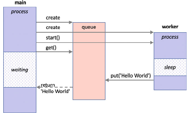
In the above diagram the main process waits for a result to be returned from the

queue following the call to the get() method; as it is waiting it is not using any

system resources. In turn the worker process sleeps for two seconds before putting

some data onto the queue (via put(‘Hello World’)). After this value is sent to

the Queue the value is returned to the main process which is woken up (moved out

of the waiting state) and can continue to process the rest of the main function.

32.9 Online Resources

See the following online resources for information discussed in this chapter:

• https://docs.python.org/3/library/threading.html for information on Thread

based barriers, locks, conditions, semaphores and events.

•

https://docs.python.org/3/library/multiprocessing.html for information on

Process based barriers, locks, conditions, semaphores and events.

•

https://en.wikipedia.org/wiki/Semaphore_p rogramming Semaphore program-

ming model.

32.10 Exercises

The aim of this exercise is to implement a concurrent version of a Stack based

container/collection.

It should be possible to safely add data to the stack and pop data off the stack

using multiple Threads.

32.8 The Concurrent Queue Class 391

It should follow a similar pattern to the Queue class described above but support

the First In Last Out (FILO) behaviour of a Stack and be usable with any number of

producer and consumer threads (you can ignore processes for this exercise).

The key to implementing the Stack is to remember that no data can be read

from the stack until there is some data to access; it is therefore necessary to wait for

data to become available and then to read it. However, it is a producer thread that

will provide that data and then inform any waiting threads that there is not data

available. You can implement this in any way you wish; however a common

solution is to use a Condition.

To illustrate this idea, the following test program can be used to verify the

behaviour of your Stack:

from stack.Stack import Stack

from time import sleep

from threading import Thread

def producer(stack):

for i in range(0,6):

data = 'Task' + str(i)

print('Producer pushing:', data)

stack.push(data)

sleep(2)

def consumer(label, stack):

while True:

print(label, 'stack.pop():', stack.pop())

print('Create shared stack')

stack = Stack()

print('Stack:', stack)

print('Creating and starting consumer threads')

consumer1 = Thread(target=consumer, args=('Consumer1', stack))

consumer2 = Thread(target=consumer, args=('Consumer2', stack))

consumer3 = Thread(target=consumer, args=('Consumer3', stack))

consumer1.start()

consumer2.start()

consumer3.start()

print('Creating and starting producer thread')

producer = Thread(target=producer, args=[stack])

producer.start()

The output generated from this sample program (which includes print statements

from the Stack) is given below:

392 32 Inter Thread/Process Synchronisation

Create shared stack

Stack: Stack: []

Creating and starting consumer threads

Creating and starting producer thread

Producer pushing: Task0

Consumer1 stack.pop(): Task0

Producer pushing: Task1

Consumer2 stack.pop(): Task1

Producer pushing: Task2

Consumer3 stack.pop(): Task2

Producer pushing: Task3

Consumer1 stack.pop(): Task3

Producer pushing: Task4

Consumer2 stack.pop(): Task4

Producer pushing: Task5

Consumer3 stack.pop(): Task5

32.10 Exercises 393

Chapter 33

Futures

33.1 Introduction

A future is a thread (or process) that promises to return a value in the future; once

the associated behaviour has completed. It is thus a future value. It provides a very

simple way of ﬁring off behaviour that will either be time consuming to execut e or

which may be delayed due to expensive operations such as Input/Output and which

could slow down the execution of other elements of a program. This chapter

discusses futures in Python.

33.2 The Need for a Future

In a normal method or function invocation, the method or function is executed in

line with the invoking code (the caller) having to wait until the function or method

(the callee) returns. Only after this is the caller able to continue to the next line of

code and execute that. In many (most) situations this is exactly what you want as

the next line of code may depend on a result returned from the previous line of code

etc.

However, in some situations the next line of code is independent of the previous

line of code. For example, let us assume that we are populating a User Interface

(UI). The ﬁrst line of code may read the name of the user from some external data

source (such as a database) and then display it within a ﬁeld in the UI. The next line

of code may then add todays data to another ﬁeld in the UI. The se two lines of code

are independent of each other and could be run concurrently/in parallel with each

other.

In this situation we could use either a Thread or a Process to run the two

lines of code independently of the caller, thus achieving a level of concurrency and

allowing the caller to carry onto the third line of code etc.

J. Hunt, Advanced Guide to Python 3 Programming,

Undergraduate Topics in Computer Science,

https://doi.org/10.1007/978-3-030-25943-3_33

395

However, neither the Thread or the Process by default provide a simple

mechanism for obtaining a resul t from such an independent operation. This may not

be a problem as operations may be self-contained; for example they may obtain data

from the database or from today’s date and then updated a UI. However, in many

situations the calculation will return a result which needs to be handled by the

original invoking code (the caller). This could involve performing a long running

calculation and then using the result returned to generate another value or update

another object etc.

A Future is an abstraction that simpliﬁes the deﬁnition and execution of such

concurrent tasks. Futures are available in many different languages including

Python but also Java, Scala, C++ etc. When using a Future; a callable object (such

as a function) is passed to the Future which executes the behaviour either as a

separate Thread or as a separate Process and then can return a result once it is

generated. The result can either be handled by a call back function (that is invoked

when the result is available) or by using a operation that will wait for a result to be

provided.

33.3 Futures in Python

The concurrent.futures library was introduced into Python in version 3.2

(and is also available in Python 2.5 onwards). The concurrent.futures

library provi des the Future class and a high level API for working with Futures.

The concurrent.futures.Future class encapsulates the asynchronous

execution of a callable object (e.g. a function or method).

The Future class provi des a range of methods that can be used to obtain

information about the state of the future, retrieve results or cancel the future:

• cancel() Attempt to cancel the Future. If the Future is currently being

executed and cannot be cancelled then the method will return False, otherwise

the call will be cancelled and the method will return True.

• cancelled() Returns True if the Future was successfully cancelled.

• running() Returns True if the Future is currently being executed and cannot

be cancelled.

• done() Returns True if the Future was successfully cancelled or ﬁnished

running.

• result(timeo ut=None) Retu rn the value returned by the Future. If the

Future hasn’t yet completed then this method will wait up to timeout seconds. If

the call hasn’t completed in timeout seconds, then a TimeoutError will be

raised. timeout can be an int or ﬂoat. If timeout is not speciﬁed or None,

there is no limit to the wait time. If the future is cancelled before completing

then the CancelledError will be raised. If the call raised, this method will

raise the same exception.

396 33 Futures

It should be noted however, that Future instances should not be created directly,

rather they should be created via the submit method of an appropriate executor.

33.3.1 Future Creation

Futures are created and executed by Executors. An Executor provides two

methods that can be used to execute a Future (or Futures) and one to shut down

the executor.

At the root of the executor class hierarchy is the concurrent.futures.

Executor abstract class. It has two subclasses:

• the ThreadPoolExecutor and

• the ProcessPoolExecutor.

The ThreadPoolExecutor uses threads to execute the futures while the

ProcessPoolExecutor uses separate processes. You can therefore choose

how you want the Future to be executed by specifying one or other of these

executors.

33.3.2 Simple Example Future

To illustrate these ideas, we will look at a very simple example of using a Future.

To do this we will use a simple worker function; similar to that used in the

previous chapters:

from time import sleep

# define function to be used with futur

def worker(msg):

for i in range(0, 10):

print(msg, end='', flush=True)

sleep(1)

return i

The only difference with this version of worker is that it also returns a result

which is the number of times that the worker printed out the message.

We can of course invoke this method inline as follows:

res = worker('A')

print(res)

33.3 Futures in Python 397

We can make the invocation of this method into a Future. To do this we use a

ThreadPoolExecutor imported from the concurrent.futures module.

We will then submit the worker function to the pool for execution. This returns a

reference to a Future which we can use to obtain the result:

from time import sleep

from concurrent.futures import ThreadPoolExecutor

print('Setting up the ThreadPoolExecutor')

pool = ThreadPoolExecutor(1)

# Submit the function ot the pool to run

# concurrently - obtain a future from pool

print('Submitting the worker to the pool')

future = pool.submit(worker, 'A')

print('Obtained a reference to the future object', future)

# Obtain the result from the future - wait if necessary

print('future.result():', future.result())

print('Done')

The output from this is:

Setting up the ThreadPoolExecutor

Submitting the worker to the pool

AAObtained a reference to the future object <Future at

0x1086ea8d0 state=running>

AAAAAAAAfuture.result(): 9

Done

Notice how the output from the main program and the worker is interwoven with

two ‘A’s being printed out before the message starting ‘Obtained a…’.

In this case a new ThreadPoolExecutor is being created with one thread in

the pool (typically there would be multiple threads in the pool but one is being used

here for illustrative purposes).

The submit() method is then used to submit the function worker with the

parameter ‘A’ to the ThreadPoolExecutor for it to schedule execution of the

function. The submit() method returns a Future object.

The main program then waits for the future object to return a result (by calling

the result() method on the future). This method can also take a timeout.

To change this example to use Processes rather than Threads all that is needed is

to change the pool executor to a ProcessPoolExecutor:

398 33 Futures

The output from this program is very similar to the last one:

Setting up the ThreadPoolExecutor

Submitting the worker to the pool

Obtained a reference to the future object <Future at

0x109178630 state=running>

AAAAAAAAAAfuture.result(): 9

Done

The only difference is that in this particular run the message starting ‘Obtained

a..’ is printed out before any of the ‘A’s are printed; this may be due to the fact that a

Process initially takes longer to set up than a Thread.

33.4 Running Multiple Futures

Both the ThreadPoolExecutor and the ProcessPoolExecutor can be

conﬁgured to support multiple Threads/Processes via the pool. Each task that is

submitted to the pool will then run within a separate Thread/Process. If more tasks

are submitted than there are Threads/Processes available, then the submitted task

will wait for the ﬁrst available Thread/Process and then be executed. This can act as

a way of managing the amount of concurrent work being done.

For example, in the following example, the worker() function is submitted to

the pool four times, but the pool is conﬁgured to use threads. Thus the fourth worker

will need to wait until one of the ﬁrst three completes before it is able to execute:

from concurrent.futures import ProcessPoolExecutor

print('Setting up the ThreadPoolExecutor')

pool = ProcessPoolExecutor(1)

print('Submitting the worker to the pool')

future = pool.submit(worker, 'A')

print('Obtained a reference to the future object', future1)

print('future.result():', future.result())

print('Done')

from concurrent.futures import ThreadPoolExecutor

print('Starting...')

pool = ThreadPoolExecutor(3)

future1 = pool.submit(worker, 'A')

future2 = pool.submit(worker, 'B')

future3 = pool.submit(worker, 'C')

future4 = pool.submit(worker, 'D')

print('\nfuture4.result():', future4.result())

print('All Done')

33.3 Futures in Python 399

When this runs we can see that the Futures for A, B and C all run concurrently

but D must wait until one of the others ﬁnishes:

Starting...

ABCACBCABCBABCACBACABCBACABCBADDDDDDDDDD

future4.result(): 9

All Done

The main thread also waits for future4 to ﬁnish as it requests the result which

is a blocking call that will only return once the future has completed and generates a

result.

Again, to use Processes rather than Threads all we need to do is to replace the

ThreadPoolExecutor with the ProcessPoolExecutor:

from concurrent.futures import ProcessPoolExecutor

print('Starting...')

pool = ProcessPoolExecutor(3)

future1 = pool.submit(worker, 'A')

future2 = pool.submit(worker, 'B')

future3 = pool.submit(worker, 'C')

future4 = pool.submit(worker, 'D')

print('\nfuture4.result():', future4.result())

print('All Done')

33.4.1 Waiting for All Futures to Complete

It is possible to wait for all futures to complete before progressing. In the previous

section it was assumed that future4 would be the last future to complete; but in

many cases it may not be possible to know which future will be the last to complete.

In such situations it is very useful to be able to wait for all the futures to complete

before continuing. This can be done using the concurrent.futures.wait

function. This funct ion takes a collection of futures and optionally a timeout and

a return_when indicator.

wait(fs, timeout=None, return_when=ALL_COMPLETED)

where:

• timeout can be used to control the maximum number of seconds to wait

before returning. timeout ca n be an int or ﬂoat. If timeout is not speciﬁed or

None, there is no limit to the wait time.

• return_when indicates when this function should retur n. It must be o ne of

the following constants:

– FIRST_COMPLETED The function will return when any future ﬁnishes or is

cancelled.

400 33 Futures

– FIRST_EXCEPTION The function will return when any future ﬁnishes by

raising an exception. If no future raises an exception, then it is equivalent to

ALL_COMPLETE D.

– ALL_COMPLETED The function will return when all futures ﬁnish or are

cancelled.

The wait() function returns two sets done and not_done. The ﬁrst set

contains the futures that completed (ﬁnished or were cancel led) before the wait

completed. The second set, the not_dones, contains uncompleted futures.

We can use the wait() function to modify out previous example so that we no

longer rely on future4 ﬁnishing last:

from concurrent.futures import ProcessPoolExecutor

from concurrent.futures import wait

from time import sleep

def worker(msg):

for i in range(0,10):

print(msg,end='', flush=True)

sleep(1)

return i

print('Starting...setting up pool')

pool = ProcessPoolExecutor(3)

futures = []

print('Submitting futures')

future1 = pool.submit(worker, 'A')

futures.append(future1)

future2 = pool.submit(worker, 'B')

futures.append(future2)

future3 = pool.submit(worker, 'C')

futures.append(future3)

future4 = pool.submit(worker, 'D')

futures.append(future4)

print('Waiting for futures to complete')

wait(futures)

print('\nAll Done')

The output from this is:

Starting...setting up pool

Submitting futures

Waiting for futures to complete

ABCABCABCABCABCABCBCACBACBABCADDDDDDDDDD

All Done

Note how each future is added to the list of futures which is then passed to the

wait() function.

33.4 Running Multiple Futures 401

33.4.2 Processing Results as Completed

What if we want to process each of the results returned by our collection of futures?

We could loop through the futures list in the previous section once all the results

have been generated. However, this means that we would have to wait for them all

to complete before processing the list.

In many situations we would like to process the results as soon as they are

generated without being concerned if that is the ﬁrst, third, last or second etc.

The concurrent.futures.as_completed() function does preciously

this; it will serve up each future in turn as soon as they are completed; with all

futures eventu ally being returned but without guaranteeing the order (just that as

soon as a future is ﬁnished generating a result it will be immediately available).

For example, in the following example, the is_even() function sleeps for a

random number of seconds (ensuring that different invocations of this function will

take different durations) then calculates a result:

The second for loop will loop through each future as they complete printing out

the result from each, as shown below:

from concurrent.futures import ThreadPoolExecutor, as_completed

from time import sleep

from random import randint

def is_even(n):

print('Checking if', n , 'is even')

sleep(randint(1, 5))

return str(n) + ' ' + str(n % 2 == 0)

print('Started')

data = [1, 2, 3, 4, 5, 6]

pool = ThreadPoolExecutor(5)

futures = []

for v in data:

futures.append(pool.submit(is_even, v))

for f in as_completed(futures):

print(f.result())

print('Done')

402 33 Futures

As you can see from this output although the six futures were started in sequence

the results returned are in a different order (with the returned order being 1, 4, 5, 3, 2

and ﬁnally 6).

33.5 Processing Future Results Using a Callback

An alternative to the as_complete() approach is to provide a function that will

be called once a result has been generated. This has the advantage that the main

program is never paused; it can continue doing whatever is required of it.

The function called once the result is generated is typically known as a callback

function; that is the future calls back to this function when the result is available.

Each future can have a separate call back as the function to invoke is set on the

future using the add_done_callback() method. This method takes the name

of the function to invoke.

For example, in this modiﬁed version of the previous example, we specify a call

back function that will be used to print the futures result. This call back function is

called print_future_result(). It takes the future that has completed as its

argument:

Started

Checking if 1 is even

Checking if 2 is even

Checking if 3 is even

Checking if 4 is even

Checking if 5 is even

Checking if 6 is even

1 False

4 True

5 False

3 False

2 True

6 True

Done

33.4 Running Multiple Futures 403

When we run this, we can see that the call back function is called after the main

thread has completed. Again, the order is unspeci ﬁed as the is_even() function

still sleeps for a random amount of time.

Started

Checking if 1 is even

Checking if 2 is even

Checking if 3 is even

Checking if 4 is even

Checking if 5 is even

Done

In callback Future result: 1 False

Checking if 6 is even

In callback Future result: 5 False

In callback Future result: 4 True

In callback Future result: 3 False

In callback Future result: 2 True

In callback Future result: 6 True

from concurrent.futures import ThreadPoolExecutor

from time import sleep

from random import randint

def is_even(n):

print('Checking if', n, 'is even')

sleep(randint(1, 5))

return str(n) + ' ' + str(n % 2 == 0)

def print_future_result(future):

print('In callback Future result: ', future.result())

print('Started')

data = [1, 2, 3, 4, 5, 6]

pool = ThreadPoolExecutor(5)

for v in data:

future = pool.submit(is_even, v)

future.add_done_callback(print_future_result)

print('Done')

404 33 Futures

33.6 Online Resources

See the following online resources for information on Future s:

•

https://docs.python.org/3/library/concurrent.futures.html The Python standard

Library documentation on Futures.

•

https://pymotw.com/3/concurrent.futures The Python Module of the Week page

on Futures.

•

https://www.blog.pythonlibrary.org/2016/08/03/python-3-concurrency-the-

concurrent-futures-module

an alternative tutorial on Python Futures.

33.7 Exercises

In mathematics, the factorial of a positive integer n, denoted by n!, is the pro-

duct of all positive integers less than or equal to n. For example,

5! = 5  4  3  2  1=120

Note that the value of 0! is 1.

Write a Future that will calculate the factorial of any number with the result

being printed out via a call back function.

There are several ways in which the factorial value can be calculated either using

a for loop or a recursive function. In either case sleep for a millisecond between

each calculation.

Start multiple Futures for different factorial values and see which comes back

ﬁrst.

33.6 Online Resources 405

Chapter 34

Concurrency with AsyncIO

34.1 Introduction

The Async IO facilities in Python are relatively recent additions originally intro-

duced in Python 3.4 and evolving up to and including Python 3.7. They are

comprised (as of Python 3.7) of two new keywords async and await (introduced

in Python 3.7) and the Async IO Python package.

In this chapter we ﬁrst discuss Asynchronous IO before introducing the async

and await keywords. We then present Async IO Tasks, how they are created used

and managed.

34.2 Asynchronous IO

Asynchronous IO (or Async IO) is a language agnostic concurrent programming

model (or paradigm) that has been implemented in several different programming

language (such as C# and Scala) as well as in Python.

Asynchronous IO is another way in which you can build concurrent applications

in Python. It is in many ways an alternative to the facilities provided by the

Threading library in Python. However, were as the Threading library is more

susceptible to issues associated with the GIL (The Gl obal Interpreter Lock) which

can affect perfor mance, the Async IO facilities are better insulated from this issue.

The way in which Async IO operates is also lighter weight then the facilities

provide day the multiprocessing library since the asynchronous tasks in

Async IO run within a single process rather than requiring separate processes to be

spawned on the underlying hardware.

Async IO is therefore another alternative way of implementing concurrent

solutions to problems. It should be noted that it does not build on either Threading

or Multi Processing; instead Async IO is based on the idea of cooperative

J. Hunt, Advanced Guide to Python 3 Programming,

Undergraduate Topics in Computer Science,

https://doi.org/10.1007/978-3-030-25943-3_34

407

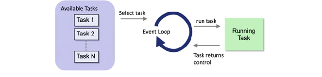
multitasking. These cooperating tasks operate asynchronously; by this we mean that

the tasks:

• are able to operate separately from other tasks,

• are able to wait for another task to return a result when required,

• and are thus able to allow other tasks to run while they are waiting.

The IO (Input/Output) aspect of the name Async IO is because this form of

concurrent program is best suited to I/O bound tasks.

In an I/O bound task a program spends most of its time sending data to, or

reading data from, some form of external device (for example a database or set of

ﬁles etc.). This communi cation is time consuming and means that the program

spends most of its time waiting for a response from the external device.

One way in which such I/O bound applications can (appear to) speed up is to

overlap the execution of different tasks; thus, while one task is waiting for a

database to respond with some data, another task can be writing data to a log ﬁle

etc.

34.3 Async IO Event Loop

When you are dev eloping code using the Async IO facilities you do not need to

worry about how the internals of the Async IO library work; however at least at the

conceptual level it is useful to understand one key concept; that of the Async IO

Event Loop; This loop controls h ow and when each task gets run. For the purposes

of this discussion a task represents some work that can be run independently of

other pieces of work.

The Event Loop knows about each task to be run and what the state of the task

currently is (for example whether it is waiting for something to happen/complete) . It

selects a task that is ready to run from the list of available tasks and executes it.

This task has complete control of the CPU until it either completes its work or

hands back control to the Event Loop (for example, because it must now wait for

some data to be supplied from a database). The Event Loop now checks to see if

any of the waiting tasks are ready to continue executing and makes a note of their

status. The Event Loop then selects another task that is ready to run and starts that

task off. This loop continues until all the tasks have ﬁnished. This is illustrated

below:

408 34 Concurrency with AsyncIO

An important point to note in the above description is that a task does not give

up the processor unless it decides to, for example by having to wait for something

else. They never get interrupted in the middle of an operation; this avoids the

problem that two threads might have when being time sliced by a separate scheduler

as they may both be sharing the same resource. This can greatly simplify your code.

34.4 The Async and Await Keywords

The async keyword, introduced in Python 3.7 is used to mark a function as being

something that uses the await keyword (we will come back to this below as there

is one other use of the async keyword). A function that uses the await keyword

can be run as a separate task and can give up control of the processor when it calls

await against another async function and must wait for that function to com-

plete. The invoked async function can then run as a separate task etc.

To invoke an async function it is necessary to start the Async IO Event Loop

and for that function to be treated as a task by the Event Loop. This is done by

calling the asyncio.run() method and passing in the root async function.

The asyncio.run() function was introduced in Python 3.7 (older versions of

Python such as Python 3.6 required you to explicitly obtain a reference to the Event

Loop and to run the root async function via that). One point to note about this

function is that it has been marked as being provisional in Python 3.7. This means

that future versions of Python may or may not support the function or may modify

the function in some way. You should therefore check the documentation for the

version of Python you are using to see whether the run method has been altered or

not.

34.4.1 Using Async and Await

We will examine a very simple Async IO program from the top down. The main()

function for the program is given below:

def main() :

print('Main - Starting')

asyncio.run(do_something())

print('Main - Done')

if __name__ == '__main__':

main()

34.3 Async IO Event Loop 409

The main() function is the entry point for the program and calls:

asyncio.run(do_something())

This starts the Async IO Event Loop running and results in the do_some-

thing() function being wrapped up in a Task that is managed by the loop. Note

that you do not explicitly create a Task in Async IO; they are always created by

some function however it is useful to be aware of Tasks as you can interact with

them to check their status or to retrieve a result.

The do_something() function is marked with the keyword async:

async def do_something():

print('do_something - will wait for worker')

result = await worker()

print('do_something - result:', result)

As previously mentioned this indicates that it can be run as a separate Task and

that it can use the keyword await to wait for some other function or behaviour to

complete. In this case the do_something() asynchronous function must wait for

the worker() function to complete.

The await keyword does more than merely indicate that the do_something

() function must wait for the worker to complete. It triggers another Task to be

created that will execute the worker() function and releases the processor

allowing the Event Loop to select the next task to execute (which may or may not

be the task running the worker() function). The status of the do_something

task is now waiting while the status of the worker() task is ready (to run).

The code for the worker task is given below:

async def worker():

print('worker - will take some time')

time.sleep(3)

print('worker - Done it')

return 42

The async keyword again indicates that this function can be run as a separate

task. However, this time the body of the function does not use the await keyword.

This is because this is a special case known as an Async IO coroutine function. This

is a function that returns a value from a Task (it is related to the idea of a standard

Python coroutine which is a data consumer).

Sadly, Computer Sc ience has many examples where the same term has been

used for different things as well as examples where different terms have been used

for the same thing. In this case to avoid confusion just stick with Async IO

coroutines are functions marked with async that can b e run as a separate task and

may call await.

410 34 Concurrency with AsyncIO

The full listing for the program is given below:

import asyncio

import time

async def worker():

print('worker - will take some time')

time.sleep(3)

print('worker - done it')

return 42

async def do_something():

print('do_something - will wait for worker')

result = await worker()

print('do_something - result:', result)

def main():

print('Main - Starting')

asyncio.run(do_something())

print('Main - Done')

if __name__ == '__main__':

main()

When this program is executed the output is:

Main - Starting

do_something - will wait for worker

worker - will take some time

worker - done it

do_something – result: 42

Main – Done

When this is run there is a pause between the two worker printouts as it sleeps.

Although it is not completely obvious here, the do_something() function

was run as one task, this task then waited when it got to the worker() function

which was run as another Task. Once the worker task completed the do_some-

thing task could continue and complete its operation. Once this happened the

Async IO Event Loop could then terminate as no further tasks were available.

34.5 Async IO Tasks

Tasks are used to execute functions marked with the async keyword concurrently.

Tasks are never created directly instead they are created implicitly via the keyword

await or through functions such as asyncio.run described above or

34.4 The Async and Await Keywords 411

asyncio.create_task(), asyncio.gather() and asyncio.as_-

completed(). These additional task creation functions are described below:

• asyncio.crea te_task() This function takes a function marked with

async and wraps it inside a Task and schedules it for execution by the

Async IO Event Loop. This function was added in Python 3.7.

• asyncio.gath er(*aws) This function runs all the async functions passed

to it as separate Tasks. It gathers the results of each separate task together and

returns them as a list. The order of the results corresponds to the order of the

async functions in the aws list.

• asyncio.as_c ompleted(aws) Runs each of the async functions passed

to it.

A Task object supports several useful methods

• cancel() cancels a running task. Calling this method will cause the Task to

throw a CancelledError exception.

• cancelled() returns Tr ue if the Task has been cancelled.

• done() returns True if the task has completed, raised an exception or was

cancelled.

• result() returns the result of the Task if it is done. If the Tasks result is not

yet available, then the method raises the InvalidStateError exception.

• exception() return an exception if one was raised by the Tas k. If the task

was cancelled then raises the CancelledError exception. If the task is not

yet done, then raises an InvalidStateError exception.

It is also possible to add a callback function to invoke once the task has com-

pleted (or to remove such a function if it has been added):

• add_done_cal lback(callback) Add a callback to be run when the

Task is done.

• remove_done_ callback(callback) Remove callback from the call-

backs list.

Note that the method is called ‘add’ rather than ‘set’ implying that there can be

multiple functions called when the task has completed (if required).

The following example illustrates some of the above:

async def worker():

print('worker - will take some time')

await asyncio.sleep(1)

print('worker - Done it')

return 42

def print_it(task):

print('print_it result:', task.result())

import asyncio

412 34 Concurrency with AsyncIO

In this example, the worker() function is wrapped within a task object that is

returned from the asyncio.create_task(worker()) call.

A function (print_it()) is registered as a callback on the task using the

asyncio.create_task(worker()) function. Note that the worker is passed

the task that has completed as a parameter. This allows it to obtain information from

the task such as any result generated.

In this example the async function do_something() explicitly waits on the

task to complete. Once this happens several different methods are used to obtain

information about the task (such as whether it was cancelled or not).

One other point to note about this listing is that in the worker() function we

have added an await using the asyncio.slee p(1) function; this allows the

worker to sleep and wait for the triggered task to complete; it is an Async IO

alternative to time.sleep(1).

The output from this program is:

Main - Starting

do_something - create task for worker

do_something - add a callback

worker - will take some time

worker - Done it

print_it result: 42

do_something - task.cancelled(): False

do_something - task.done(): True

do_something - task.result(): 42

do_something - task.exception(): None

do_something - finished

Main - Done

async def do_something():

print('do_something - create task for worker')

task = asyncio.create_task(worker())

print('do_something - add a callback')

task.add_done_callback(print_it)

await task

# Information on task

print('do_something - task.cancelled():',

task.cancelled())

print('do_something - task.done():', task.done())

print('do_something - task.result():', task.result())

print('do_something - task.exception():',

task.exception())

print('do_something - finished')

def main() :

print('Main - Starting')

asyncio.run(do_something())

print('Main - Done')

if __name__ == '__main__':

main()

34.5 Async IO Tasks 413

34.6 Running Multiple Tasks

In many cases it is useful to be able to run several tasks concurrently. There are

two options provided for this the asyncio.gather() and the asyncio.

as_completed() function; we will look at both in this section.

34.6.1 Collating Results from Multiple Tasks

It is often useful to collect all the results from a set of tasks together and to continue

only once all the results have been obtained. When using Threads or Processes this

can be achieved by starting multiple Threads or Processes and then using some

other object such as a Barrier to wait for all the results to be available before

continuing. Within the Async IO library all that is required is to use the asyn-

cio.gather() funct ion with a list of the async functions to run, for example:

import asyncio

import random

async def worker():

print('Worker - will take some time')

await asyncio.sleep(1)

result = random.randint(1,10)

print('Worker - Done it')

return result

async def do_something():

print('do_something - will wait for worker')

# Run three calls to worker concurrently and collect

results

results = await asyncio.gather(worker(), worker(),

worker())

print('results from calls:', results)

def main() :

print('Main - Starting')

asyncio.run(do_something())

print('Main - Done')

if __name__ == '__main__':

main()

In this program the do_something( ) function uses

results = await asyncio.gather(worker(), worker(), worker())

to run three invocations of the worker() function in three separate Tasks and to

wait for the results of all three to be made available before they are returned as a list

of values and stored in the results variable.

414 34 Concurrency with AsyncIO

This makes is very easy to work with multiple concurrent tasks and to collate

their results.

Note that in this code example the worker async function returns a random

number between 1 and 10.

The output from this program is:

do_something - will wait for worker

Worker - will take some time

Worker - Done it

results from calls: [5, 3, 4]

Main – Done

Main - Starting

As you can see from this all three of the worker invocations are started but then

release the processor while they sleep. After this the three tasks wake up and

complete before the results are collected together and printed out.

34.6.2 Handling Task Results as They Are Made Available

Another option when running multiple Tasks is to handle the results as they become

available, rather than wait for all the results to be provided before continuing. This

option is supported by the asyncio.as_completed() function. This function

returns an iterator of async functions which will be served up as soon as they have

completed their work.

The for-loop construct can be used with the iterator returned by the function;

however within the for loop the code must call await on the async functions

returned so that the result of the task can be obtained. For example:

async def do_something():

print('do_something - will wait for worker')

# Run three calls to worker concurrently and collect

results

for async_func in asyncio.as_completed((worker('A'),

worker('B'),

worker('C'))):

result = await async_func

print('do_something - result:', result)

Note that the asyncio.as_completed() function takes a container such as

a tuple of async functions.

34.6 Running Multiple Tasks 415

We have also modiﬁed the worker function slightly so that a label is added to the

random number generated so that it is clear which invocation of the worker function

return which result:

async def worker(label):

print('Worker - will take some time')

await asyncio.sleep(1)

result = random.randint(1,10)

print('Worker - Done it')

return label + str(result)

When we run this program

def main() :

print('Main - Starting')

asyncio.run(do_something())

print('Main - Done')

The output is

Main - Starting

do_something - will wait for worker

Worker - will take some time

Worker - Done it

do_something - result: C2

do_something - result: A1

do_something - result: B10

Main – Done

As you can see from this, the results are not returned in the order that the tasks

are created, task ‘C’ completes ﬁrst followed by ‘A’ and ‘B’. This illustrates the

behaviour of the asyncio.as_completed() function.

34.7 Online Resources

See the following online resources for information on Futures:

•

https://docs.python.org/3/library/asyncio-task.html The Python standard Library

documentation on AsyncIO.

•

https://pymotw.com/3/asyncio The Python Module of the Week page on

AsyncIO.

•

https://pythonprogramming.net/asyncio-basics-intermediate-python-tutorial An

AsyncIO tutorial.

416 34 Concurrency with AsyncIO

34.8 Exercises

This exercise will use the facilities in the AsyncIO library to calculate a set of

factorial numbers.

The factorial of a positive integer is the product of all positive integers less than

or equal to n. For example,

5! = 5 x 4 x 3 x 2 x 1 = 120

Note that the value of 0! is 1,

Create an application that will use the async and await keywords to calculate

the factorials of a set of numbers. The factorial function should await for 0.1 of a

second (using asyncio.slee p(0.1)) each time round the loop used to cal-

culate the factorial of a number.

You can use with asyncio.as_completed() or asyncio.gather() to

collect the results up.

You might also use a list comprehension to create the list of calls to the factorial

function.

The main function might look like:

def main():

print('Main - Starting')

asyncio.run(calculate_factorials([5, 7, 3, 6]))

print('Main - Done')

if __name__ == '__main__':

main()

34.8 Exercises 417

Part VIII

Reactive Programming

Chapter 35

Reactive Programming Introduction

35.1 Introduction

In this chapter we will introduce the concept of Reactive Programming. Reactive

programming is a way of write programs that allow the system to reactive to data

being published to it. We will look at the RxPy library which provides a Python

implementation of the ReactiveX approach to Reactive Programming.

35.2 What Is a Reactive Application?

A Reactive Application is one that must react to data; typically either to the

presence of new data, or to changes in existing data. The Reactive Manifesto

presents the key characteristics of Reactive Systems as:

• Responsive. This means that such systems respond in a timely manner. Here of

course timely will differ depending upon the application and domain; in one

situation a second may be timely in another it may be far too slow.

• Resilient. Such systems stay responsive in the face of failure. The systems must

therefore be desig ned to handle fail ure gracefully and continue to work

appropriately following the failure.

• Elastic. As the workload grows the system should continue to be responsive.

• Message Driven. Information is exchanged between elements of a reactive

system using messages. This ensures loose coupling, isolation and location

transparency between these components.

As an example, consider an application that lists a set of Equity Stock Trade

values based on the latest market stick price data. This application might present the

current value of each trade within a table. When new market stock price data is

J. Hunt, Advanced Guide to Python 3 Programming,

Undergraduate Topics in Computer Science,

https://doi.org/10.1007/978-3-030-25943-3_35

421

published, then the application must update the value of the trade within the table.

Such an application can be described as being reactive.

Reactive Programming is a programming style (typically supported by libraries)

that allows code to be written that follow the ideas of reactive systems. Of course

just because part of an application uses a Reactive Programming library does not

make the whole application reactive; indeed it may only be necessary for part of an

application to exhibit reactive behaviour.

35.3 The ReactiveX Project

ReactiveX is the best known implementation of the Reactive Programming

paradigm.

ReactiveX is based on the Observer-Observable design pattern. However it is an

extension to this design pattern as it extends the pattern such that the approach

supports sequences of data and/or events and adds operators that allow developers

to compose sequences together declaratively while abstracting away concerns

associated with low-level threads, synchronisatio n, concurrent data structures and

non-blocking I/O.

The ReactiveX project has implementations for many languages including

RxJava, RxScala and RxPy; this last is the version we are looking at as it is for the

Python language.

RxPy is described as:

A library for composing asynchronous and event-based programs using Observable col-

lections and query operator functions in Python

35.4 The Observer Pattern

The Observer Pattern is one of the Gang of Four set of Design Patterns. The Gang

of Four Patterns (as originally described in Gamma et al.

1995) are so called

because this book on design patterns was written by four very famous authors

namely; Erich Gamma, Richard Helm, Ralph Johnso n and John Vlissides.

The Observer Pattern provides a way of ensuring that a set of objects is notiﬁed

whenever the state of another object changes. It has been widely used in a number

of languages (such as Smalltalk and Java) and can also be used with Python.

The intent of the Observer Pattern is to manage a one to many relationship

between an object and those objects interested in the state, and in particular state

changes, of that object. Thus when the objects’ state changes, the interested (de-

pendent) objects are notiﬁed of that change and can take whatever action is

appropriate.

422 35 Reactive Programming Introduction

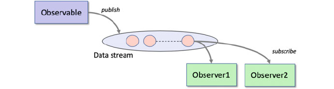
There are two key roles within the Observer Pattern, these are the Observable

and the Observer roles.

• Observable. This is the object that is responsible for notifying other objects that

a change in its state has occurred

• Observer. An Observer is an object that will be noti ﬁed of the change in state of

the Observable and can take appropriate action (such as triggering a change in

their own state or performing some action).

In addition the state is typically represented explicitly:

• State. This role may be played by an object that is used to share information

about the change in state that has occurred within the Observable. This might be

as simple as a String indicating the new state of the Observable or it might be a

data oriented object that provides more detailed information.

These roles are illustrated in the following ﬁgure.

In the above ﬁgure, the Observable object publishes data to a Data Stream. The

data in the Data Stream is then sent to each of the Observers registered with the

Observable. In this way data is broadcast to all Observers of an Observable.

It is common for an Observable to only publish data once there is an Observer

available to process that data. The process of registering with an Observable is

referred to as subscribing. Thus an Observable will have zero or more subscribers

(Observers).

If the Observable publishes data at a fast er rate than can be processed by the

Observer then the data is queued via the Data Stream. This allows the Observer to

process the data received one at a time at its own pace; without any concern for data

loss (as long as sufﬁcient memory is available for the data stream).

35.5 Hot and Cold Observables

Another concept that it is useful to understand is that of Hot and Cold Observables.

• Cold Observables are lazy Observables. That is, a Cold Observable will only

publish data if at least one Observer is subscribed to it.

35.4 The Observer Pattern 423

• Hot Observables, by contrast, publish data whether there is an Observer sub-

scribed or not.

35.5.1 Cold Observables

A Cold Observable will not publish any data unless there is at least one Observer

subscribed to process that data. In addition a cold Observable only provides data to

an Observer when that Observer is ready to process the data; this is because the

Observable-Observer relationship is more of a pull relationship. For example, given

an Observable that will generate a set of values based on a range, then that

Observable will generate each result lazily when requested by an Observer.

If the Observer takes some time to process the data emitted by the Observable,

then the Observable will wait until the Observer is ready to process the data before

emitting another value.

35.5.2 Hot Observables

Hot Observables by contrast publish data whether there is an Observer subscribed

or not. When an Observer registers with the Observable, it will start to receive data

at that point, as and when the Observable publishes new data. If the Observable has

already published previous data items, then these will have been lost and the

Observer will not receive that data.

The most common situation in which a Hot Observable is created is when the

source producer represents data that may be irrelevant if not processed immediately

or may be superseded by subsequent data. For example, data published by a Stock

Market Price data feed would fall into this category. W hen an Observable wraps

around this data feed it can publish that data whether or not an Observer is

subscribed.

35.5.3 Implications of Hot and Cold Observables

It is important to know whether you have a hot or cold Observable because this can

impact on what you can assume about the data supplied to the Observers and thus

how you need to design your application. If it is important that no data is lost then

care is needed to ensure that the subscribers are in place before a Hot Observable

starts to publish data (where as this is not a concern for a cold Observable).

424 35 Reactive Programming Introduction

35.6 Differences Between Event Driven Programming

and Reactive Programming

In Event Driven programming, an event is generated in response too something

happening; the event then represents this with any associated data. For example, if

the user clicks the mouse then an associated MouseClickEvent might be

generated. This object will usually hold information about the x and y coordinates

of the mouse along with which button was clicked etc. It is then possi ble to

associate some behaviour (such as a function or a method) with this event so that if

the event occurs, then the associated operation is invoked and the event object is

provided as a parameter. This is certainly the approach used in the wxPython

library presented earlier in this book:

From the above diagram, when a MoveEvent is generated the on_move()

method is called and the event is passed into the method.

In the Reactive Programming approach, an Observer is associated with an

Observable. Any data generated by the Observable will be received and handled by

the Observer. This is true whatever that data is, as the Observer is a handler of data

generated by the Observable rather than a handler of a speciﬁc type of data (as with

the Event driven approach).

Both approaches could be used in many situations. For example, we could have

a scenario in which some data is to be processed whenever a stock price changes.

This could be implemented using a StockPriceChangeEvent associated

with a StockPriceEventHandler. It could also be implemented via Stock

PriceChangeObserverable and a StockPriceChangeObserver.In

either case one element handles the data generated by another element. However,

the RxPy library simpliﬁes this process and allows the Observer to run in the same

thread as, or a separate thread from, the Observable with just a small change to the

code.

35.7 Advantages of Reactive Programming

There are several advantages to the use of a Reactive Programming library these

include:

• It avoids multiple callback methods. The problems associated with the use of

callbacks are sometimes referred to as callback hell. This can occur when there

are multiple callbacks, all deﬁned to run in response to some data being gen-

erated or some operation completing. It can be hard to understand, maintain and

debug such systems.

35.6 Differences Between Event Driven Programming and Reactive Programming 425

• Simpler asynchronous, multi threaded execution. The approach adopted by

RxPy makes it very easy to execute operations/ behaviour within a multi

threaded environment with independent asynchronous functions.

• Available Operators. The RxPy library comes pre built with numerous oper-

ators that make processing the data produced by an Observable much easier.

• Data Composition. It is straight forward to compose new data streams

(Observables) from data supplied by two or more other Observables for asyn-

chronous processing.

35.8 Disadvantages of Reactive Programming

Its easy to over complicate things when you start to chain operators together. If you

use too many operators, or too complex a set of functions with the operators, it can

become hard to understand what is going on.

Many developers think that Reactive programming is inherently multi-threaded;

this is not necessarily the case; in fact RxPy (the library explored in the next two

chapters) is single threaded by default. If an application needs the behaviour to

execute asynchronously then it is necessary to explicitly indicate this.

Another issue for some Reactive programming frameworks is that it can become

memory intensive to store streams of data so that Observers can proces ses that data

when they are ready.

35.9 The RxPy Reactive Programming Framework

The RxPy library is a part of the larger ReactiveX project and provides an

implementation of ReactiveX for Python. It is built on the concepts of Observables,

Observers, Subjects and operators. In this book we use RxPy version 3.

In the next chapter we will discuss Observables, Observers, Subjects and sub-

scriptions using the RxPy library. The following chapter will explore various RxPy

operators.

35.10 Online Resources

See the following online resources for information on reactive programming:

•

https://www.reactivemanifesto.org/ The Reactive Manifesto.

•

http://reactivex.io/ The ReactiveX home page.

•

https://en.wikipedia.org/wiki/Design_Patterns Wikipedia page on Design

Patterns book.

426 35 Reactive Programming Introduction

35.11 Reference

For more information on the Observer Observable design pattern see the “Patterns”

book by the Gang of Four

• E. Gamma, R. Helm, R. Johnson, J. Vlissades, Design patterns: elements of

reusable object-oriented software, Addison-Wesley (1995).

35.11 Reference 427

Chapter 36

RxPy Observables, Observers

and Subjects

36.1 Introduction

In this chapter we will discuss Observables, Observers and Subjects. We also

consider how observers may or may not run concurrently.

In the remainder of this chapter we look at RxPy version 3 which is a major

update from RxPy version 1 (you will therefore need to be careful if you are

looking on the web for examples as some aspects have changed; most notably the

way in which operators are chained).

36.2 Observables in RxPy

An Observable is a Python class that publishes data so that it can be processed

by one or more Observers (potentially running in separate threads).

An Observable can be created to publish data from static data or from

dynamic sources. Observables can be chained tougher to control how and when

data is published, to transform data before it is published and to restrict what data is

actually published.

For example, to create an Observable from a list of values we can use the

rx.from_list() function. This function (also know n as an RxPy operator) is

used to create the new Observable object:

import rx

Observable = rx.from_list([2, 3, 5, 7])

J. Hunt, Advanced Guide to Python 3 Programming,

Undergraduate Topics in Computer Science,

https://doi.org/10.1007/978-3-030-25943-3_36

429

36.3 Observers in RxPy

We can add an Observer to an Observable using the subcribe() method.

This method can be supplied with a lambda function, a named function or an object

whose class implements the Observer protocol .

For example, the simplest way to create an Observer is to use a lambda function:

# Subscribe a lambda function

observable.subscribe(lambda value: print('Lambda Received',

value))

When the Observable publishes data the lambda function will be invoked.

Each data item published will be supplied independently to the function. The output

from the above subscription for the previous Observable is:

Lambda Received 2

Lambda Received 3

Lambda Received 5

Lambda Received 7

We can also have used a standard or named function as an Observer:

def prime_number_reporter(value):

print('Function Received', value)

# Subscribe a named function

observable.subscribe(prime

number

reporter)

Note that it is only the name of the function that is used with the subscribe()

method (as this effectively passes a reference to the function into the method).

If we now run this code using the previous Observable we get:

Function Received 2

Function Received 3

Function Received 5

Function Received 7

In actual fact the subscribe() method takes four optional parameters. Thes

are:

• on_next Action to invoke for each data item generated by the Observable.

• on_error Action to invoke upon exceptional termination of the Observable

sequence.

• on_completed Action to invoke upon graceful termination of the Observable

sequence.

• Observer The object that is to receive notiﬁcations. You may subscribe using

an Observer or callbacks, not both.

430 36 RxPy Observables, Observers and Subjects

Each of the above can be used as position al parameters or as keyword argu-

ments, for example:

# Use lambdas to set up all three functions

observable.subscribe(

on_next = lambda value: print('Received on_next', value),

on_error = lambda exp: print('Error Occurred', exp),

on_completed = lambda: print('Received completed

notification')

)

The above code deﬁnes three lambda functions that will be called depending

upon whether data is supplied by the Observable, if an error occurs or when the

data stream is terminated. The output from this is:

Received on_next 2

Received on_next 3

Received on_next 5

Received on_next 7

Received completed notification

Note that the on_error function is not run as no error was generated in this

example.

The ﬁnal optional parameter to the subscribe() method is an Observer

object. An Observer object can implement the Observer protocol which has the

following methods on_next(), on_completed() and on_error(), for

example:

class PrimeNumberObserver:

def on_next(self, value):

print('Object Received', value)

def on_completed(self):

print('Data Stream Completed')

def on_error(self, error):

print('Error Occurred', error)

Instances of this class can now be used as an Observer via the subscribe()

method:

observable.subscribe(PrimeNumberObserver())

# Subscribe an Observer object

The output from this example using the previous Observable is:

Object Received 2

Object Received 3

Object Received 5

Object Received 7

Data Stream Completed

Note that the on_completed() method is also call ed; however the

on_errror() method is not called as there were no exceptions generated.

36.3 Observers in RxPy 431

The Observer class must ensure that the methods implemented adhere to the

Observer protocol (i.e. That the signatures of the on_next(), on_completed

() and on_error() methods are correct).

36.4 Multiple Subscribers/Observers

An Observable can have multiple Observers subscribed to it. In this case each of the

Observers is sent all of the data published by the Observable. Multiple Observers

can be registered with an Observable by calling the subscribe method multiple

times. For example, the following program has four subscribers as well as

on_error and on_completed function registered:

# Create an observable using data in a list

observable = rx.from_list([2, 3, 5, 7])

class PrimeNumberObserver:

""" An Observer class """

def on_next(self, value):

print('Object Received', value)

def on_completed(self):

print('Data Stream Completed')

def on_error(self, error):

print('Error Occurred', error)

def prime_number_reporter(value):

print('Function Received', value)

print('Set up Observers / Subscribers')

# Subscribe a lambda function

observable.subscribe(lambda value: print('Lambda Received',

value))

# Subscribe a named function

observable.subscribe(prime_number_reporter)

# Subscribe an Observer object

observable.subscribe(PrimeNumberObserver())

# Use lambdas to set up all three functions

observable.subscribe(

on_next=lambda value: print('Received on_next', value),

on_error=lambda exp: print('Error Occurred', exp),

on_completed=lambda: print('Received completed

notification')

)

432 36 RxPy Observables, Observers and Subjects

The output from this program is:

Create the Observable object

Set up Observers / Subscribers

Lambda Received 2

Lambda Received 3

Lambda Received 5

Lambda Received 7

Function Received 2

Function Received 3

Function Received 5

Function Received 7

Object Received 2

Object Received 3

Object Received 5

Object Received 7

Data Stream Completed

Received on_next 2

Received on_next 3

Received on_next 5

Received on_next 7

Received completed notification

Note how each of the subscribers is sent all of the data before the next subscriber

is sent their data (this is the default single threaded RxPy behaviour).

36.5 Subjects in RxPy

A subject is both an Observer and an Observable. This allows a subject to receive

an item of data and then to republish that data or data derived from it.

For example, imagine a subject that recei ves stock market price data published

by an external (to the organi sation receiving the data) source. This subject might

add a timestamp and source location to the data before republishing it to other

internal Observers.

However, there is a subtle difference that should be noted between a Subject and

a plain Observable . A subscription to an Observable will cause an independent

execution of the Observable when data is published. Notice how in the previous

section all the messages wer e sent to a speciﬁc Observer before the next Observer

was sent any data at all.

However, a Subject shares the publication action with all of the subscribers and

they will therefore all receive the same data item in a chain before the next data

item.

In the class hierarchy the Subject class is a direct subclass of the Observer

class.

36.4 Multiple Subscribers/Observers 433

The following example creates a Subject that enriche s the data it receives by

adding a timestam p to each data item. It then republishes the data item to any

Observers that have subscribed to it.

import rx

from rx.subjects import Subject

from datetime import datetime

source = rx.from_list([2, 3, 5, 7])

class TimeStampSubject(Subject):

def on_next(self, value):

print('Subject Received', value)

super().on_next((value, datetime.now()))

def on_completed(self):

print('Data Stream Completed')

super().on_completed()

def on_error(self, error):

print('In Subject - Error Occurred', error)

super().on_error(error)

def prime_number_reporter(value):

print('Function Received', value)

print('Set up')

# Create the Subject

subject = TimeStampSubject()

# Set up multiple subscribers for the subject

subject.subscribe(prime_number_reporter)

subject.subscribe(lambda value: print('Lambda Received',

value))

subject.subscribe(

on_next = lambda value: print('Received on_next', value),

on_error = lambda exp: print('Error Occurred', exp),

on_completed = lambda: print('Received completed

notification')

)

# Subscribe the Subject to the Observable source

source.subscribe(subject)

print('Done')

Note that in the above program the Observers are added to the Subject before

the Subject is added to the source Observable. This ensures that the Observers

are subscribed before the Subject starts to receive data published by the

434 36 RxPy Observables, Observers and Subjects

Observable. If the Subje ct was subscribed to the Observable before the

Observers were subscribed to the Subject, then all the data could have been

published before the Observers were registered with the Subject.

The output from this program is:

Set up

Subject Received 2

Function Received (2, datetime.datetime(2019, 5, 21, 17, 0, 2,

196372))

Lambda Received (2, datetime.datetime(2019, 5, 21, 17, 0, 2,

196372))

Received on_next (2, datetime.datetime(2019, 5, 21, 17, 0, 2,

196372))

Subject Received 3

Function Received (3, datetime.datetime(2019, 5, 21, 17, 0, 2,

196439))

Lambda Received (3, datetime.datetime(2019, 5, 21, 17, 0, 2,

196439))

Received on_next (3, datetime.datetime(2019, 5, 21, 17, 0, 2,

196439))

Subject Received 5

Function Received (5, datetime.datetime(2019, 5, 21, 17, 0, 2,

196494))

Lambda Received (5, datetime.datetime(2019, 5, 21, 17, 0, 2,

196494))

Received on_next (5, datetime.datetime(2019, 5, 21, 17, 0, 2,

196494))

Subject Received 7

Function Received (7, datetime.datetime(2019, 5, 21, 17, 0, 2,

196548))

Lambda Received (7, datetime.datetime(2019, 5, 21, 17, 0, 2,

196548))

Received on_next (7, datetime.datetime(2019, 5, 21, 17, 0, 2,

196548))

Data Stream Completed

Received completed notification

Done

As can be seen from this output the numbers 2, 3, 5 and 7 are received by all of

the Observers once the Subject has added the timestamp.

36.6 Observer Concurrency

By default RxPy uses a single threaded model; that is Observables and Observers

execute in the same thread of execution. However, this is only the default as it is the

simplest approach.

It is possible to indicate that when a Observer subscribes to an Observable that it

should run in a separate thread using the scheduler keyword parameter on the

36.5 Subjects in RxPy 435

subscribe() method. This keyword is given an appropriate scheduler such as

the rx.concurrency.NewThreadScheduler. This scheduler will ensure

that the Observer runs in a separate thread.

To see the difference look at the following two programs. The main difference

between the programs is the use of speciﬁc schedulers:

import rx

Observable = rx.from_list([2, 3, 5])

observable.subscribe(lambda v: print('Lambda1 Received', v))

observable.subscribe(lambda v: print('Lambda2 Received', v))

observable.subscribe(lambda v: print('Lambda3 Received', v))

The output from this ﬁrst version is given below:

Lambda1 Received 2

Lambda1 Received 3

Lambda1 Received 5

Lambda2 Received 2

Lambda2 Received 3

Lambda2 Received 5

Lambda3 Received 2

Lambda3 Received 3

Lambda3 Received 5

The subscribe() method takes an optional keyword parameter called

scheduler that allows a scheduler object to be provided.

Now if we specify a few different schedulers we will see that the effect is to run

the Observers concurrently with the resultin g output being interwoven:

import rx

from rx.concurrency import NewThreadScheduler,

ThreadPoolScheduler, ImmediateScheduler

Observable = rx.from_list([2, 3, 5])

observable.subscribe(lambda v: print('Lambda1 Received', v),

scheduler=ThreadPoolScheduler(3))

observable.subscribe(lambda v: print('Lambda2 Received', v),

scheduler=ImmediateScheduler())

observable.subscribe(lambda v: print('Lambda3 Received', v),

scheduler=NewThreadScheduler())

# As the Observable runs in a separate thread need

# ensure that the main thread does not terminate

input('Press enter to finish')

436 36 RxPy Observables, Observers and Subjects

Note that we have to ensure that the main thread running the program does not

terminate (as all the Observables are now running in their own threads) by waiting

for user input. The output from this version is:

Lambda2 Received 2

Lambda1 Received 2

Lambda2 Received 3

Lambda2 Received 5

Lambda1 Received 3

Lambda1 Received 5

Press enter to finish

Lambda3 Received 2

Lambda3 Received 3

Lambda3 Received 5

By default the sched uler keyword on the subscribe() method defaults to

None indicating that the current thread will be used for the subscription to the

Observable.

36.6.1 Available Schedulers

To support different scheduling strategi es the RxPy library provides two

modules that supply different schedulers; the rx.concurrency and rx.

currency.mainloopscheduler. The modules contain a variety of sched-

ulers including those listed below.

The following schedulers are available in the rx.concurrency module:

• ImmediateSch eduler This schedules an action for immediate execution.

• CurrentThrea dScheduler This schedules activity for the current thread.

• TimeoutSched uler This scheduler works via a timed callback.

• NewThreadSch eduler creates a scheduler for each unit of work on a sep-

arate thread.

• ThreadPoolSc heduler. This is a scheduler that utilises a thread pool to

execute work. This scheduler can act as a way of throttling the amount of work

carried out concurrently.

The rx.concurrency.mainloopschduler module also deﬁnes the fol-

lowing schedulers:

• IOLoopSchedu ler A scheduler that schedules work via the Tornado I/O

main event loop.

• PyGameSchedu ler A scheduler that schedules works for PyGame.

• WxScheduler A scheduler for a wxPython event loop.

36.6 Observer Concurrency 437

36.7 Online Resources

See the following online resources for information on RxPy:

•

https://github.com/ReactiveX/RxPY The RxPy Git hub repository.

•

https://rxpy.readthedocs.io/en/latest/ Document ation for the RxPy library.

•

https://rxpy.readthedocs.io/en/latest/operators.html Lists of the available RxPy

operators.

36.8 Exercises

Given the following set of tuples representing Stock/Equity prices:

stocks = (('APPL', 12.45), ('IBM', 15.55), ('MSFT', 5.66),

('APPL', 13.33))

Write a program that will create an Observable based on the stocks data.

Next subscribe three different observers to the Observable. The ﬁrst should print

out the stock price, the second should print out the name of the stock and the third

should print out the entire tuple.

438 36 RxPy Observables, Observers and Subjects

Chapter 37

RxPy Operators

37.1 Introduction

In this chapter we will look at the types of operators provided by RxPy that can be

applied to the data emitted by an Observable.

37.2 Reactive Programming Operators

Behind the interaction between an Observable and an Observer is a data stream.

That is the Observable supplies a data stream to an Observer that consumes/

processes that stre am. It is possible to apply an operator to this data stream that can

be used to to ﬁlter, transform and generally reﬁn e how and when the data is

supplied to the Observer.

The operators are mostly deﬁned in the rx.operators module, for example

rx.operators.average(). However it is common to use an alias for this

such that the operators module is called op, such as

from rx import operators as op

This allows for a short hand form to be used when referencing an operator, such

as op.average().

Many of the RxPy operators execute a function which is applied to each of the

data items produced by an Observable. Others can be used to create an initial

Observable (indeed you have already seen these operators in the form of the

from_list() operator). Another set of operators can be used to generate a result

based on data produced by the Observable (such as the sum() operator).

J. Hunt, Advanced Guide to Python 3 Programming,

Undergraduate Topics in Computer Science,

https://doi.org/10.1007/978-3-030-25943-3_37

439

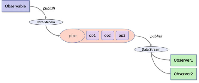
In fact RxPy provides a wide variety of operators and these operators can be

categorised as follows:

• Creational,

• Transformational,

• Combinatorial,

• Filters,

• Error handlers,

• Conditional and Boolean operators,

• Mathematical,

• Connectable.

Examples of some of these categories are presented in the rest of this section.

37.3 Piping Operators

To apply an operator other than a creational operator to an Observable it is nec-

essary to create a pipe. A Pipe is essentially a series of one or more operations that

can be applied to the data stream generated by the Observable. The result of

applying the pipe is that a new data stream is generated that represents the results

produced following the application of each operator in turn. This is illustrated

below:

To create a pipe the Observable.pipe() method is used. This method takes

a comma delimited list of one or more operat ors and returns a data stream.

Observers can then subscribe to the pipe’s data stream. This can be seen in the

examples given in the rest of this chapter for transformations, ﬁlters, mathematical

operators etc.

440 37 RxPy Operators

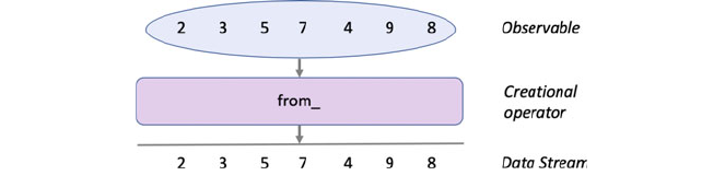
37.4 Creational Operators

You have already seen an example of a creational operator in the examples pre-

sented earlier in this chapter. This is because the rx.from_list() operator is an

example of a creational operator. It is used to create a new Observable based on

data held in a list like structure.

A more generic version of from_list() is the from_() operator. This

operator takes an iterable and generates an Observable based on the data provided

by the iterable. Any object that implements the iterable protocol can be used

including user deﬁned types. There is also an operator from_iterable(). All

three operators do the same thing and you can choose which to use based on which

provides the most semantic meaning in your context.

All three of the following statements have the same effect:

source = rx.from_([2, 3, 5, 7])

source = rx.from_iterable([2, 3, 5, 7])

source = rx.from_list([2, 3, 5, 7])

This is illustrated pictorially below:

Another creational operator is the rx.range() operator. This operator gen-

erates an observable for a range of integer numbers. The range can be speciﬁed with

our without a starting value and with or within an increment. However the maxi-

mum value in the range must always be provided, for example:

obs1 = rx.range(10)

obs2 = rx.range(0, 10)

obs3 = rx.range(0, 10, 1)

37.5 Transformational Operators

There are several transformati onal operators deﬁned in the rx.operators

module including rx.operators.map() and rx.operators.ﬂat_map().

The rx.operators.map() operator applies a function to each data item

generated by an Observable.

37.4 Creational Operators 441

The rx.operators.ﬂat_map() operator also applies a function to each

data item but then applies a ﬂatten operation to the result. For example, if the result

is a list of lists then ﬂat_map will ﬂatten this into a single list. In this section we

will focus on the rx.operators.map() operator.

The rx.operators.map() operator allows a function to be applied to all

data items generated by an Observable. The result of this function is then returned

as the result of the map() operators Observable. The function is typically used to

perform some form of transformation to the data supplied to it. This could be

adding one to all integer values, converting the format of the data from XML to

JSON, enriching the data with additional information such as the time the data was

acquired and who the data was supplied by etc.

In the example given below we are transforming the set of integer values sup-

plied by the original Observable into strings. In the diagram these strings

include quotes around them to highlight they are in fact a string:

This is typical of the use of a transformation operator; that is to change the data

from one format to another or to add information to the data.

The code used to implement this scenario is given below. Note the use of the

pipe() method to apply the operator to the data stream generated by the

Observable:

# Apply a transformation to a data source to convert

# integers into strings

import rx

from rx import operators as op

# Set up a source with a map function

source = rx.from_list([2, 3, 5, 7]).pipe(

op.map(lambda value: "'" + str(value) + "'")

)

# Subscribe a lambda function

source.subscribe(lambda value: print('Lambda Received',

value,

' is a string ',

isinstance(value, str)))

442 37 RxPy Operators

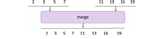
The output from this program is:

Lambda Received '2' is a string True

Lambda Received '3' is a string True

Lambda Received '5' is a string True

Lambda Received '7' is a string True

37.6 Combinatorial Operators

Combinatorial operators combine together multiple data items in some way. One

example of a combinatorial operator is the rx.merge() operator. This operator

merges the data produced by two Observables into a single Observable data stream.

For example:

In the above diagram two Observables are represented by the sequence 2, 3, 5, 7

and the sequence 11, 13, 16, 19. The se Observables are supplied to the merge

operator that generates a single Observable that will supply data generat ed from

both of the original Observables. This is an example of an operator that does not

take a function but instead takes two Observables.

The code representing the above scenario is given below:

# An example illustrating how to merge two data source

import rx

# Set up two sources

source1 = rx.from_list([2, 3, 5, 7])

source2 = rx.from_list([10, 11, 12])

# Merge two sources into one

rx.merge(source1, source2)\

.subscribe(lambda v: print(v, end=','))

Notice that in this case we have subscribed directly to the Observable returned

by the merge() operator and have not stored this in an intermediate variable (this

was a design decision and either approach is acceptable).

37.5 Transformational Operators 443

The output from this program is presented below:

2,3,5,7,10,11,12,

Notice from the output the way in which the data held in the original Observables

is intertwined in the output of the Observable generated by the merge() operator.

37.7 Filtering Operators

There are several operators in this category including rx.operators.ﬁlter

(), rx.operators.ﬁrst(), rx.operators.last() and rx.opera-

tors.distinct().

The ﬁlter() operator only allows those data items to pass through that pass

some test expression deﬁned by the function passed into the ﬁlter. This function

must return True or False. Any data item that causes the function to return True

is allowed to pass through the ﬁlter.

For example, let us assume that the function passed into ﬁlter() is designed

to only allow even numbers through. If the data stream contains the numbers 2, 3, 5,

7, 4, 9 and 8 then the ﬁlter() will only emit the numbers 2, 4 and 8. This is

illustrated below:

The following code implements the above scenario:

# Filter source for even numbers

import rx

from rx import operators as op

# Set up a source with a filter

source = rx.from_list([2, 3, 5, 7, 4, 9, 8]).pipe(

op.filter(lambda value: value % 2 == 0)

)

# Subscribe a lambda function

source.subscribe(lambda value: print('Lambda Received', value))

In the above code the rx.operators.ﬁlter() operator takes a lambda

function that will verify if the current value is even or not (note this could have been

a named function or a method on an object etc.). It is applied to the data stream

generated by the Observable using the pipe() method. The output generated by

this example is:

444 37 RxPy Operators

Lambda Received 2

Lambda Received 4

Lambda Received 8

The ﬁrst() and last() operators emit only the ﬁrst and last data item

published by the Observable.

The distinct() operator suppresses duplicate items being published by the

Observable. For example, in the following list used as the data for the Observable,

the numbers 2 and 3 are duplicated:

# Use distinct to suppress duplicates

source = rx.from_list([2, 3, 5, 2, 4, 3, 2]).pipe(

op.distinct()

)

# Subscribe a lambda function

source.subscribe(lambda value: print('Received', value))

However, when the output is generated by the program all duplicates have been

suppressed:

Received 2

Received 3

Received 5

Received 4

37.8 Mathematical Operators

Mathematical and aggregate operators perform calculations on the data stream

provided by an Observable. For example, the rx.operators.average()

operator can be used to calculate the average of a set of numbers published by an

Observable. Similarly rx.operators.max() can select the maximum value,

rx.operators.min() the minimum value and rx.operators.sum() will

total all the numbers published etc.

An example using the rx.operators.sum() operator is given blow:

# Example of summing all the values in a data strea

import rx

from rx import operators as op

# Set up a source and apply sum

rx.from_list([2, 3, 5, 7]).pipe(

op.sum()

).subscribe(lambda v: print(v))

37.7 Filtering Operators 445

The output from the rx.operato rs.sum() operator is the total of the data

items published by the Observable (in this case the total of 2, 3, 5 and 7). The

Observer function that is subscribed to the rx.operators.sum() operators

Observable will print out this value:

However, in some cases it may be useful to be notiﬁed of the intermediate

running total as well as the ﬁnal value so that other operators down the chain can

react to these subtotals. This can be achieved using the rx.operators.scan()

operator. The rx.operators.scan() operator is actually a transformational

operator but can be used in this case to provide a mathematical operation. The

scan() operator applies a function to each data item published by an Observable

and generates its own data item for each value received. Each generated value is

passed to the next invoca tion of the scan() function as well as being published to

the scan() operators Observable data stream. The running total can thus be

generated from the previous sub total and the new value obtained. This is shown

below:

import rx

from rx import operators as op

# Rolling or incremental sum

rx.from_([2, 3, 5, 7]).pipe(

op.scan(lambda subtotal, i: subtotal+i)

).subscribe(lambda v: print(v))

The output from this example is:

This means that each subtotal is published as well as the ﬁnal total.

37.9 Chaining Operators

An interest ing aspect of the RxPy approach to data stream processing is that it is

possible to apply multiple operators to the data stream produced by an Observable.

The operators discussed earlier actually return another Observable. This new

Observable can supply its own data stream based on the original data stream and the

result of applying the operator. This allows another operator to be applied in

sequence to the data produced by the new Observable. This allows the operators to

be chained toget her to provide sophisticated processing of the data published by the

original Observable.

446 37 RxPy Operators

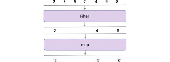
For example, we might ﬁrst start off by ﬁltering the output from an Observable

such that only certain data items are published. We might then apply a transfor-

mation in the form of a map() operator to that data, as shown below:

Note the the order in which we have applied the operators; we ﬁrst ﬁlter out data

that is not of interest and then apply the transformation. This is more efﬁcient than

apply the operators the other way around as in the above example we do not need to

transform the odd values. It is therefore common to try a nd push the ﬁlter operators

as high up the chain as possible.

The code used to generate the chained set of operators is given below. In this

case we have used lambda functions to deﬁne the ﬁlter() function and the map

() function. The operators are applied to the Observable obtained from the list

supplied. The data stream generated by the Observable is processed by each of the

operators deﬁned in the pipe. As there are now two operators the pipe contains both

operators and acts a pipe down which the data ﬂows.

The list used as the initial source of the Observables data contains a sequence of

event and odd numbers. The ﬁlter() function selects only even numbers and the

map() function transforms the integer values into strings. We then subscribe an

Observer function to the Observable produced by the transformational map()

operator.

# Example of chaining operators together

import rx

from rx import operators as op

# Set up a source with a filter

source = rx.from_list([2, 3, 5, 7, 4, 9, 8])

pipe = source.pipe(

op.filter(lambda value: value % 2 == 0),

op.map(lambda value: "'" + str(value) + "'")

)

# Subscribe a lambda function

pipe.subscribe(lambda value: print('Received', value))

37.9 Chaining Operators 447

The output from this application is given below:

Received '2'

Received '4'

Received '8'

This makes it clear that only the three even numbers (2, 4 and 8) are allowed

through to the map() function.

37.10 Online Resources

See the following online resources for information on RxPy:

•

https://rxpy.readthedocs.io/en/latest/ Document ation for the RxPy library.

•

https://rxpy.readthedocs.io/en/latest/operators.html Lists of the available RxPy

operators.

37.11 Exercises

Given the following set of tuples representing Stock/Equity prices:

stocks = (('APPL', 12.45), ('IBM', 15.55), ('MSFT', 5.66),

('APPL', 13.33))

Provide solutions to the following:

• Select all the ‘APPL’ stocks

• Select all stocks with a price over 15.00

• Find the average price of all ‘APPL’ stocks.

Now use the second set of tuples and merge them with the ﬁrst set of stock

prices:

stocks2 = (('GOOG', 8.95), ('APPL', 7.65), ('APPL', 12.45),

('MSFT', 5.66), ('GOOG', 7.56), ('IBM', 12.76))

Convert each tuple into a list and calculate how much 25 shares in that stock

would be, print this out as the result).

• Find the highest value stock.

• Find the lowest value stock.

• Only publish unique data times (I.e. Suppress duplicates).

448 37 RxPy Operators

Part IX

Network Programming

Chapter 38

Introduction to Sockets and Web

Services

38.1 Introduction

In the following two chapters we will explore socket based and web service

approaches to inter process communications. These processes may be running on

the same computer or different computers on the same local area network or may be

geographically far apart. In all cases information is sent by one program running in

one process to another program running in a separate process via internet sockets.

This chapter introduces the core concepts involved in network programming.

38.2 Sockets

Sockets, or rather Internet Protocol (IP) sockets provide a programming interface to

the network protocol stack that is managed by the underlying operating system.

Using such an API means that the programmer is abstracted away from the low

level details of how data is exchanged between process on (potentially) different

computers and can instead focus on the higher level aspects of their solution.

There are a number of different types of IP socket available, however the focus

in this book is on Stream Sockets. A stream socket uses the Transmission Control

Protocol (TCP) to send messages. Such a socket is often referred to as a TCP/IP

socket.

TCP provides for ordered and reliable transmission of data across the connection

between two devices (or hosts). This can be important as TCP guarantees that for

every message sent; that every message will not only arrive at the receiving host but

that the messages will arrive in the correct order.

A common alternative to the TCP is the User Datagram Protocol (or UDP). UDP

does not provide any delivery guarantees (that is messages can be lost or may arrive

out of order). However, UDP is a simpler protocol and can be particularly useful for

J. Hunt, Advanced Guide to Python 3 Programming,

Undergraduate Topics in Computer Science,

https://doi.org/10.1007/978-3-030-25943-3_38

451

broadcast systems, where multiple clients may need to receive the data published by

a server host (particularly if data loss is not an issue).

38.3 Web Services

A Web Service is a service offered by a host computer that can be invoked by a

remote client using the Hypertext Transfer Protocol (HTTP). HTTP can be run over

any reliable stream transport protocol, although it is typically used over TCP/IP. It

was originally designed to allow data to be transferred between a HTTP server and

a web browser so that the data could be presented in a human readable form to a

user. However, when used with a web service it is used to support program to

program communication between a client and a server using machine-readable data

formats. Currently this format is most typically JSON (Java Script Object Notation)

although in the past XML (eXtensible Markup Language) was often used.

38.4 Addressing Services

Every device (host) connected to the internet has a unique identity (we are ignoring

private networks here). This unique identity is represented as an IP address. Using

an IP address we can connect a socket to a speciﬁc host anywhere on the internet. It

is therefore possible to connect to a whole range of device types in this way from

printers to cash tills to fridges as well as servers, mainframes and PCs etc.

IP addresses have a common format such as 144.124.16.237. An IP version

4 address is always a set of four numbers separated by full stops. Each number can

be in the range 0–255, so the full range of IP addresses is from 0.0.0.0 to

255.255.255.255.

An IP address can be divided up into two parts; the part indicating the network

on which the host is connected and the host’s ID, for example:

Thus:

• The Network ID elements of the IP addres s identiﬁes the speciﬁc network on

which the host is currently located.

• The Host ID is the part of the IP address that speciﬁes a speciﬁcities device on

the network (such as your computer).

452 38 Introduction to Sockets and Web Services

On any given network there may be multiple hosts, each with their own host ID

but with a shared network ID. For example, on a private home network there may

be:

• 192.168.1.1 Jasmine’s laptop.

• 192.168.1.2 Adam’ sPC

• 192.168.1.3 Home Printer

• 192.168.1.4 Smart TV

In many ways the network id and host id elements of an IP address are like the

postal address for a house on a street. The street may have a name, for example

Coleridge Avenue and there may be multiple houses on the street. Each house has a

unique number; thus 10 Coleridge Avenue is uniquely differentiated from 20

Coleridge Avenue by the house number.

At this point you may be wondering where the URLs you see in your web

browser come into play (such as

www.bbc.co.uk). These are textual names that

actually map to an IP address. The mapping is performed by something called a

Domain Name System (or DNS) server. A DNS server acts as a lookup service to

provide the actual IP addres s for a particular textual URL name. The presence of an

english textual version of a host address is because humans are better at remem-

bering (a hopefully) meaningful name rather than what might appear to be a random

sequence of numbers.

There are several web sites that can be used to see these mappings (and one is

given at the end of this chapter). Some examples of how the english textual name

maps to an IP address are given below:

•

www.aber.ac.uk maps to 144.124.16.237

•

www.uwe.ac.uk maps to 164.11.132.96

•

www.bbc.net.uk maps to 212.58.249.213

•

www.gov.uk maps to 151.101.188.144

Note that these mappings were correct at the time of writing; they can change as

new entries can be provided to the DNS servers causing a particular textual name to

map to a different physical host.

38.5 Localhost

There is a special IP address which is usually available on a host computer and is

very useful for developers and testers. This is the IP address:

It is also known as localhost which is often easier to remember.

127.0.0.1

38.4 Addressing Services 453

Localhost (and 127.0.0.1) is used to refer to the computer you are currently

on when a program is run; that is it is your local host computer (hence the name

localhost).

For examp le, if you start up a socket server on your local computer and want a

client socket program, running on the same computer, to connect to the server

program; you can tell it to do so by getting it to connect to localhost.

This is particularly useful when either you don’t know the IP address of your

local computer or because the code may be run on multiple different computers

each of which will have their own IP address. This is particularly common if you

are writing test code that will be used by developers when running their own tests

on different developer (host) machines.

We will be using localhost in the next two chapters as a way of specifying where

to look for a server program.

38.6 Port Numbers

Each internet device/host can typically support multiple processes. It is therefore

necessary to ensure that each process has its own channel of communications. To

do this each host has available to it multiple ports that a program can connect too.

For example port 80 is often reserved for HTTP web servers, while port 25 is

reserved for SMTP servers. This means that if a client wants to connect to a HTTP

server on a particular computer then it must specify port 80 not port 25 on that host.

A port number is written after the IP address of the host and separated from the

address by a colon, for example:

•

www.aber.ac.uk:80 indicates port 80 on the host machine which will typically

be running a HTTP server, in this case for Aberystwyth University.

• localhost:143 this indicates that you wish to connect to port 143 which is

typically reserved for an IMAP (Internet Message Access Protocol) server on

your local machine.

•

www.uwe.ac.uk:25 this indicates port 25 on a host running at the University of

the West of England, Bristol. Port 25 is usually reserved for SMTP (Simple Mail

Transfer Protocol) servers.

Port numbers in the IP system are 16 bit numbers in the range 0–65 536.

Generally, port numbers below 1024 are reserved for pre-deﬁned services (which

means that you should avoid using them unless you wish to communicate with one

of those services such as telnet, SMTP mail, ftp etc.). Therefore it is typically to

choose a port number above 1024 when setting up your won services.

454 38 Introduction to Sockets and Web Services

38.7 IPv4 Versus IPv6

What we have described in this chapter in terms of IP addresses is in fact based on

the Internet Protocol version 4 (aka IPv4). This version of the Internet Protocol was

developed during the 1970s and published by the IETF (Internet Engineering Task

Force) in September 1981 (replacing an earlier deﬁnition published in January

1980). This version of the standard uses 32 binary bits for each element of the host

address (hence the range of 0 to 255 for each of there parts of the address). This

provides a total of 4.29 billion possible unique addresses. This seemed a huge

amount in 1981 and certainly enough for what was imagined at the time for the

internet.

Since 1981 the internet has become the backbone to not only the World Wide

Web itself, but also to the concept of the Internet of Things (in which every possible

device might be connected to the internet from your fridge, to your central heating

system to your toaster). This potential explosion in internet addressable devices/

hosts lead in the mid 1990as to concerns about the potential lack of internet

addresses using IPv4. The IETF therefore designed a new version of the Internet

Protocol; Internet Protocol version 6 (or IPv6). This was ratiﬁed as an Internet

Standard in July 2017.

IPv6 uses a 128 bit address for each element in a hosts address. It also uses eight

number groups (rather than 4) which are separated by a colon. Each number group

has four hexadecimal digits.

The following illustrates what an IPv6 address looks like:

Uptake of the IPv6 protocol has been slower than was originally expected, this is

in part because the IPv4 and IPv6 have not been designed to be interoperable but

also because the utilisation of the IPv4 addresses has not been as fast as many

originally feared (partly due to the use of private networks). However, over time

this is likely to change as more organisations move over to using the IPv6.

38.8 Sockets and Web Services in Python

The next two chapters discuss how sockets and web services can be implemented in

Python. The ﬁrst chapter discusses both general sockets and HTTP server sockets.

The second chapter looks at how the Flask library can be used to create web

services that run over HTTP using TCP/IP sockets.

2001:0DB8:AC10:FE01:EF69:B5ED:DD57:2CLE

38.7 IPv4 Versus IPv6 455

38.9 Online Resources

See the following online resources for information

•

https://en.wikipedia.org/wiki/Network_socket Wikipedia page on Sockets.

•

https://en.wikipedia.org/wiki/Web_service Wikipedia page on Web Services.

•

https://codebeautify.org/website-to-ip-address Provides mappings from URLs to

IP addresses.

•

https://en.wikipedia.org/wiki/IPv4 Wikipedia page on IPv4.

•

https://en.wikipedia.org/wiki/IPv6 Wikipedia page on IPv6.

•

https://www.techopedia.com/deﬁnition/28503/dn s-server For an introduction to

DNS.

456 38 Introduction to Sockets and Web Services

Chapter 39

Sockets in Python

39.1 Introduction

A Socket is an end point in a communication link between separate processes. In

Python sockets are objects which provide a way of exchanging information

between two processes in a straight forward and platform independent manner.

In this chapter we will introdu ce the basic idea of socket communications and

then presents a simple socket server and client application.

39.2 Socket to Socket Communication

When two operating system level processes wish to communicate, they can do so

via sockets. Each process has a socket which is connected to the others socket. One

process can then write information out to the socket, while the second process can

read information in from the socket.

Associated with each socket are two streams, one for input and one for output.

Thus, to pass information from one process to another, you write that information

out to the output stream of one socket object and read it from the input stream of

another socket object (assuming the two sockets are connected).

Several different types of sockets are available, however in this chapter we will

focus on TCP/IP sockets. Such a socket is a connection-oriented socket that will

provide a guarantee of delivery of data (or notiﬁcation of the failure to deliver the

data). TCP/IP, or the Transmission Control Protocol/Internet Protocol, is a suite of

communication protocols used to interconnect network devices on the internet or

in a private intranet. TCP/IP actually speciﬁes how data is exchanged between

programs over the internet by providing end-to-end communications that identify

how the data should be broken down into packets, addressed, transmitted, routed

and received at the destination.

J. Hunt, Advanced Guide to Python 3 Programming,

Undergraduate Topics in Computer Science,

https://doi.org/10.1007/978-3-030-25943-3_39

457

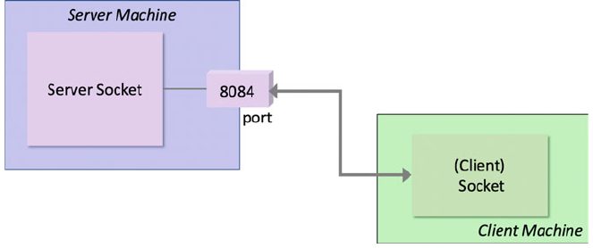
39.3 Setting Up a Connection

To set up the connection, one process must be running a program that is waiting for

a connection while the other must try to connect up to the ﬁrst program. The ﬁrst is

referred to as a server socket while the second just as a socket.

For the second process to connect to the ﬁrst (the server socket) it must know

what machine the ﬁrst is running on and which port it is connected to.

For example, in the above diagram the server socket connects to port 8084. In

turn the client socket connects to the machine on which the server is executing and

to port number 8084 on that machine.

Nothing happens until the server socket accepts the connection. At that point the

sockets are connected, and the socket streams are bound to each other. This means

that the server’s output stream is connected to the Client socket input stream and

vice versa.

39.4 An Example Client Server Application

39.4.1 The System Structure

The above diagram illustrates the basic structure of the system we are trying to

build. There will be a server object running on one machine and a client object

running on another. The client will connect up to the server using sockets in order

to obtain information.

The actual application being implemented in this example, is an address book

look up application. The addresses of employees of a company are held in a

dictionary. This dictionary is set up in the server program but could equally be held

in a database etc. When a client connects up to the server it can obtain an

employees’ ofﬁce address.

458 39 Sockets in Python

39.4.2 Implementing the Server Application

We shall describe the server application ﬁrst. This is the Python a pplication pro-

gram that will service requests from client applications. To do this it must provide a

server socket for clients to connect to. This is done by ﬁrst binding a server socket

to a port on the server machine. The server program must then listen for incoming

connections.

The listing presents the source code for the Server program.

import socket

def main():

# Setup names and offices

addresses = {'JOHN': 'C45',

'DENISE': 'C44',

'PHOEBE': 'D52',

'ADAM': 'B23'}

print('Starting Server')

print('Create the socket')

sock = socket.socket(socket.AF_INET,

socket.SOCK_STREAM)

print('Bind the socket to the port')

server_address = (socket.gethostname(),

8084)

print('Starting up on', server_address)

sock.bind(server_address)

# specifies the number of connections allowed

print('Listen for incoming connections')

sock.listen(1)

while True:

print('Waiting for a connection')

connection, client_address =

sock.accept()

39.4 An Example Client Server Applic ation 459

The Server in the above listing sets up the addresses to contain a Dictionary

of the names and addresses.

It then waits for a client to connect to it. This is done by creating a socket and

binding it to a speciﬁc port (in this case port 8084) using:

print('Create the socket')

sock = socket.socket(socket.AF_INET,

socket.SOCK_STREAM)

print('Bind the socket to the port')

server_address = (socket.gethostname(),

8084)

The construction of the socket object is discussed in more detail in the next

section.

Next the server listens for a connection from a client. Note that the sock.

listen() method takes the value 1 indicating that it will handle one connection

at a time.

An inﬁnite loop is then set up to run the server. When a connection is made from

a client, both the connection and the client address are made available. While there

is data available from the client, it is read using the recv function. Note that the data

received from the client is assumed to be a string. This is then used as a key to look

the address up in the address Dictionary.

try:

print('Connection from',

client_address)

while True:

data =

connection.recv(1024).decode()

print('Received: ', data)

if data:

key = str(data).upper()

response = addresses[key]

print('sending data back

to the client: ',

response)

connection.sendall(

response.encode())

else:

print('No more data from',

client_address)

break

finally:

connection.close()

if __name__ == '__main__':

main()

460 39 Sockets in Python

Once the address is obtained it can be sent back to the client. In Python 3 it is

necessary to decode() and encoded() the string format to the raw data

transmitted via the socket streams.

Note you should always close a socket when you have ﬁnished with it.

39.5 Socket Types and Domains

When we created the socket class above, we passed in two arguments to the socket

constructor:

socket(socket.AF_INET, socket.SOCK_STREAM)

To understand the two values passed into the socket() constructor it is

necessary to understand that Sockets are characterised according to two properties;

their domain and their type.

The domain of a socket essentially deﬁnes the communications protocols that are

used to transfer the data from one process to another. It also incorporates how

sockets are named (so that they can be referred to when establishing the

communication).

Two standard domains are available on Unix systems; these are AF_UNIX

which represents intra-system communications, where data is moved from process

to process through kernel memory buffers. AF_INET represents communication

using the TCP/IP protocol suite; in which processes may be on the same machine or

on different machines.

• A socket’s type indicates how the data is transferred through the socket. There

are essentially two options here:

• Datagram which sockets support a message-based model where no connection

is involved, and communication is not guaranteed to be reliable.

• Stream sockets that support a virtual circuit model, where data is exchange d as a

byte stream and the connection is reliable.

Depending on the domain, further socket types may be available, such as those

that support message passing on a reliable connection.

39.6 Implementing the Client Application

The client application is essentially a very simple program that creates a link to the

server application. To do this it creat es a socket object that connects to the servers’

host machine, and in our case this socket is connected to port 8084.

Once a connection has been made the client can then send the encoded message

string to the server. The server will then send back a response which the client must

decode. It then closes the connection.

39.4 An Example Client Server Application 461

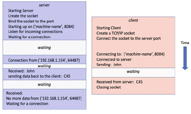
The implementation of the client is given below:

def main():

print('Starting Client')

print('Create a TCP/IP socket')

sock = socket.socket(socket.AF_INET,

socket.SOCK_STREAM)

print('Connect the socket to the server port')

server_address = (socket.gethostname(),

8084)

print('Connecting to: ', server_address)

sock.connect(server_address)

print('Connected to server')

try:

print('Send data')

message = 'John'

print('Sending: ', message)

sock.send(message.encode())

data = sock.recv(1024).decode()

print('Received from server: ', data)

finally:

print('Closing socket')

sock.close()

if __name__ == '__main__':

main()

import socket

The output from the two programs needs to be considered together.

462 39 Sockets in Python

As you can see from this diagram, the server waits for a connection from the

client. When the client connects to the server; the server waits to receive data from

the client. At this point the client must wait for data to be sent to it from the server.

The server then sets up the response data and sends it back to the client. The client

receives this and prints it out and closes the connection. In the meantime, the server

has been waiting to see if there is any more data from the client; as the client closes

the connection the server knows that the client has ﬁnished and returns to waiting

for the next connection.

39.7 The Socketserver Module

In the above example, the server code is more complex than the client; and this is

for a single threaded server; life can become much more complicated if the server is

expected to be a multi-threaded server (that is a server that can handle multiple

requests from different clients at the same time).

However, the serversocket module provides a more convenient,

object-oriented approach to creating a server. Much of the boiler plate code needed

in such applications is deﬁned in classes, with the developer only having to provide

their own classes or override methods to deﬁne the speciﬁc functionality required.

There are ﬁve different server classes deﬁned in the socketserver module.

• BaseServer is the root of the Server class hierarchy; it is not really intended

to be instantiated and used directly. Instead it is extended by TCPServer and

other classes.

• TCPServer uses TCP/IP sockets to communicate and is probably the most

commonly used type of socket server.

• UDPServer provides access to datagram sockets.

• UnixStreamSe rver and UnixDatagramServer use Unix-domain

sockets and are only available on Unix platforms.

Responsibility for processing a request is split between a server class and a

request handler class. The server deals with the communication issues (listening on

a socket and port, accepting connections, etc.) and the request handler deals with

the request issues (interpreting incoming data, processing it, sending data back to

the client).

This division of responsibility means that in many cases you can simply use one

of the existing server classes without any modiﬁcations and provide a custom

request handler class for it to work with.

The following example deﬁnes a request handler that is plugged into the

TCPServer when it is constructed. The request handler deﬁnes a method han-

dle() that will be expected to handle the request processing.

39.6 Implementing the Client Application 463

Note that the previous client application does not need to change at all; the server

changes are hidden from the client.

However, this is still a single threaded server. We can very simply make it into a

multi-threaded server (one that can deal with multiple requests concurrently) by

mixing the socketserver.ThreadingMixIn into the TCPServer. This can

be done by deﬁning a new class that is nothing more than a class that extends both

import socketserver

class MyTCPHandler(socketserver.BaseRequestHandler):

"""

The RequestHandler class for the server.

"""

def __init__(self, request, client_address, server):

print('Setup names and offices')

self.addresses = {'JOHN': 'C45',

'DENISE': 'C44',

'PHOEBE': 'D52',

'ADAM': 'B23'}

super().__init__(request, client_address, server)

def handle(self):

print('In Handle')

# self.request is the TCP socket connected

# to the client

data = self.request.recv(1024).decode()

print('data received:', data)

key = str(data).upper()

response = self.addresses[key]

print('response:', response)

# Send the result back to the client

self.request.sendall(response.encode())

def main():

print('Starting server')

server_address = ('localhost', 8084)

print('Creating server')

server =

socketserver.TCPServer(server_address,

MyTCPHandler)

print('Activating server')

server.serve_forever()

if __name__ == '__main__':

main()

464 39 Sockets in Python

ThreadingMixIn and TCPServer and creating an instane of this new class

instead of the TCPServer directly. For example:

class ThreadedEchoServer(

socketserver.ThreadingMixIn,

socketserver.TCPServer):

pass

def main():

print('Starting')

address = ('localhost', 8084)

server = ThreadedEchoServer(address,

MyTCPHandler)

print('Activating server')

server.serve_forever()

In fact you do not even need to create your own class (such as the

ThreadedEchoServer) as the socketserver.ThreadingTCPServer

has been provided as a default mixing of the TCPServer and the

ThreadingMixIn classes. We could therefore just write:

def main():

print('Starting')

address = ('localhost', 8084)

server = socketserver.ThreadedEchoServer(address,

MyTCPHandler)

print('Activating server')

server.serve_forever()

39.8 HTTP Server

In addition to the TCPServer you also have available a http.server.

HTTPServer; this can be used in a similar manner to the TCPServer, but is

used to create servers that respond to the HTTP protocol used by web browsers. In

other words it can be used to create a very simple Web Server (although it should be

noted that it is really only suitable for creating test web servers as it only imple-

ments very basic security checks).

It is probably worth a short aside to illustrate how a web server and a web

browser interact. The following diagram illustrates the basic interactions:

39.7 The Socketserver Module 465

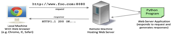
In the above diagram the user is using a browser (such as Chrome, IE or Safari)

to access a web server. The browser is running on their local machine (which could

be a PC, a Mac, a Linux box, an iPad, a Smart Phone etc.).

To access the web server they enter a URL (Universal Resource Locator) address

into their browser. In the example this is the URL

www.foo.com. It also indicates

that they want to connect up to port 8080 (rather than the default port 80 used for

HTTP connections). The remote machine (which is the one indicated by the address

www.foo.com) receives this request and determines what to do with it. If there is no

program monitoring port 8080 it will reject the request. In our case we have a

Python Program (which is actually the web server program) listening to that port

and it is passed the request. It will then handle this request and generate a response

message which will be sent back to the browser on the users local machine. The

response will indicate which version of the HTTP protocol it supports, whether

everything went ok or not (this is the 200 code in the above diagram - you may have

seen the code 404 indicating that a web page was not found etc.). The browser on

the local machine then renders the data as a web page or handles the data as

appropriate etc.

To create a simple Python web server the http.server.HTTPServer can

be used directly or can b e subclassed along with the socketserver.

ThreadingMixIn to create a multi-threaded web server, for example:

class ThreadingHTTPServer(ThreadingMixIn, HTTPServer):

"""Simple multi-threaded HTTP server """

pass

Since Python 3.7 the http.server module now provides exactly this class as

a built in facility and it is thus no longer necessary to deﬁne it yourself (see http.

server.ThreadingHTTPServer).

To handle HTTP requests you must implement one of the HTTP request

methods such as do_GET(), or do_POST() . Each of these maps to a type of

HTTP request, for example:

• do_GET() maps to a HTTP Get request that is generated if you type a web

address into the URL bar of a web browser or

• do_POST() maps to a HTTP Post request that is used for example, when a

form on a web page is used to submit data to a web server.

The do_GET(self) or do_POST(self) method must then handle any

input supplied with the request and generate any appropriate responses back to the

browser. This means that it must follow the HTTP protocol.

466 39 Sockets in Python

The following short program creates a simple web server that will generate a

welcome message and the current time as a response to a GET request. It does this

by using the datetime module to create a time stamp of the date and time using

the today() function. This is converted into a byte array using the UTF-8

character encoding (UTF-8 is the most widely used way to represent text within

web pages). We need a byte array as that is what will be executed by the write()

method later on.

Having done this there are various items of meta data that need to be set up so

that the browser knows what data it is about to receive. This meta data is known as

header data and can including the type of content being sent and the amount of data

(content) being transmitted. In our very simple case we need to tell it that we are

sending it plain text (rather than the HTML used to describe a typical web page) via

the ‘Content-type’ header information. We also need to tell it how much data we are

sending using the content length. We can then indicate that we have ﬁnished

deﬁning the header information and are now sending the actual data.

The data itself is sent via the wﬁle attribute inherited from the

BaseHTTPRequestHandler. There are infact two related attributes rﬁle and

wﬁle:

• rﬁle this is an input stream that allo ws you to read input data (which is not

being used in this example).

• wﬁle holds the output stream that can be used to write (send) data to the

browser. This object provides a method write() that takes a byte-like object

that is written out to (eventually) the browser.

A main() method is used to set up the HTTP server which follows the pattern

used for the TCPServer; however the client of this server will be a web browser.

from http.server import BaseHTTPRequestHandler,

ThreadingHTTPServer

from datetime import datetime

class MyHttpRequestHandler(BaseHTTPRequestHandler):

"""Very simple request handler. Only supports GET."""

def do_GET(self):

print("do_GET() starting to process request")

welcome_msg = 'Hello From Server at ' +

str(datetime.today())

byte_msg = bytes(welcome_msg, 'utf-8')

self.send_response(200)

self.send_header("Content-type", 'text/plain; charset-

tf-8')

39.8 HTTP Server 467

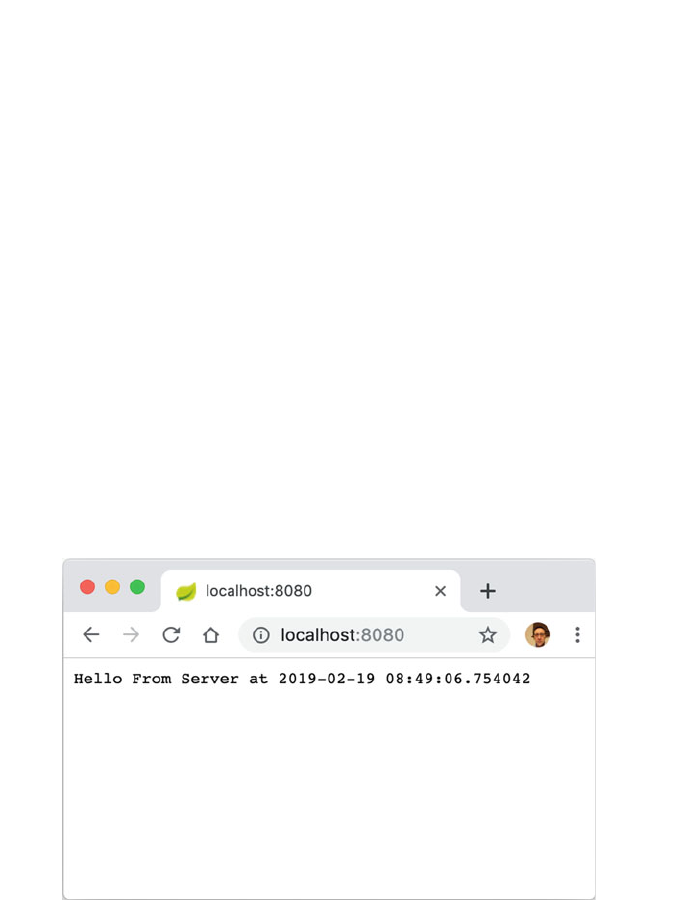
Once the server is up and running, it is possible to connect to the server using a

browser and by entering an appropriate web address into the browsers’ URL ﬁeld.

This means that in your browser (assuming it is running on the same machine as the

above program) you only need to type into the URL bar http://local-

host:8080 (this indicates you want to use the http protocol to connect up to the

local machine at port 8080).

When you do this you should see the welcome message with the current date and

time:

self.end_headers()

print('do_GET() replying with message')

self.wfile.write(byte_msg)

def main():

print('Setting up server')

server_address = ('localhost', 8080)

httpd = ThreadingHTTPServer(server_address,

MyHttpRequestHandler)

print('Activating HTTP server')

httpd.serve_forever()

if __name__ == '__main__':

self.send_header('Content-length', str(len(byte_msg)))

main()

468 39 Sockets in Python

39.9 Online Resources

See the following online resources for information on the topics in this chapter:

•

https://docs.python.org/3/howto/sockets.html tutorial on programming sockets

in Python.

•

https://pymotw.com/3/socket/tcp.html the Python Module of the Week TCP

page.

•

https://pymotw.com/3/socketserver/index.h tml The Python Module of the Week

page on SocketServer.

• https://docs.python.org/3/library/http.server.html HTTP Servers Python

documentation.

• https://pymotw.com/3/http.server/index.htm l The Python Module of the Week

page on the http.server module.

• https://www.redbooks.ibm.com/pubs/pdfs/redbooks/gg243376.pdf a PDF tuto-

rial book from IBM on TCP/IP.

•

http:// ask.pocoo.org/ for more information the Flask micro framework for web

development.

•

https://www.djangoproject.com/ provides information on the Django framework

for creating web applications.

39.10 Exercises

The aim of this exercise is to explore working with TCP/IP sockets.

You should create a TCP server that will receive a string from a client.

A check should then be made to see what information the string indicates is

required, supported inputs are:

• ‘Date’ which should result in the current date being returned.

• ‘Time’ which should result in the current time being returned.

• ‘Date and Time’ which should result in the current date and time being

returned.

• Anything else should result in the input string being returned to the client in

upper case with the message ‘UNKNOWN OPTION ’: preceding the string.

The result is then sent back to the client.

You should then create a client program to call the server. The client program

can request input from the user in the form of a string and submit that string to the

server. The result returned by the server should be displ ayed in the client before

prompting the user for the next input. If the user enters -1 as input then the program

should terminate.

39.9 Online Resources 469

An example of the type of output the client might generate is given below to

illustrate the general aim of the exercise:

Starting Client

Please provide an input (Date, Time, DataAndTime or -1 to

exit): Date

Connected to server

Sending data

Received from server: 2019-02-19

Closing socket

Please provide an input (Date, Time, DataAndTime or -1 to

exit): Time

Connected to server

Sending data

Received from server: 15:50:40

Closing socket

Please provide an input (Date, Time, DataAndTime or -1 to

exit): DateAndTime

Connected to server

Sending data

Received from server: 2019-02-19 15:50:44.720747

Closing socket

Please provide an input (Date, Time, DataAndTime or

-1 to

exit):

-1

470 39 Sockets in Python

Chapter 40

Web Services in Python

40.1 Introduction

This chapter looks at RESTful web services as implemented using the Flask

framework.

40.2 RESTful Services

REST stands for Representational State Transfer and was a termed coined by Roy

Fielding in his Ph.D. to describe the lightweight, resource-oriented architectural

style that underpins the web. Fielding, one of the principle authors of HTTP, was

looking for a way of generalising the operation of HTTP and the web. The gen-

eralised the supply of web pages as a form of data supplied on demand to a client

where the client holds the current state of an exchange. Based on this state infor-

mation the client requests the next item of relevant data sending all information

necessary to identify the information to be supplied with the request. Thus the

requests are indepe ndent and not part of an on-going stateful conversation (hence

state transfer).

It should be noted that although Fielding was aiming to create a way of

describing the pattern of behaviour withi n the web, he also had an eye on producing

lighter weight web based services (than those using either proprietary Enterprise

Integration frameworks or SOAP based services). These lighter weight HTTP based

web services have become very popular and are now widely used in many areas.

Systems which follow these principles are termed RESTful services.

A key aspect of a RESTful service is that all interactions between a client

(whether some JavaScript running in a browser or a standalone application) are

done using simple HTTP based operations. HTTP supports four operations these

are HTTP Get, HTTP Post, HTTP Put and HTTP Delete. These can be used as

J. Hunt, Advanced Guide to Python 3 Programming,

Undergraduate Topics in Computer Science,

https://doi.org/10.1007/978-3-030-25943-3_40

471

verbs to indicate the type of action being requested. Typically these are used as

follows:

• retrieve information (HTTP Get),

• create information (HTTP Post),

• update information (HTTP Put),

• delete information (HTTP Delete).

It should be noted that REST is not a standard in the way that HTML is a

standard. Rather it is a design pattern that can be used to create web applications

that can be invoked o ver HTTP and that give meaning to the use of Get, Post, Put

and Delete HTTP operations with respect to a speciﬁc resource (or type of data).

The advantage of using RESTful services as a technology, compared to some

other approaches (such as SOAP based services which can also be invoked over

HTTP) is that

• the implementations tend to be simpler,

• the maintenance easier,

• they run over standard HTTP and HTTPS protocols and

• do not require expensive infrastructures and licenses to use.

This means that there is lower server and server side costs. There is little vendor

or technology dependency and clients do not need to know anything about the

implementation details or technologies being used to create the services.

40.3 A RESTful API

1. A RESTful API is one in which you must ﬁrst determin e the key concepts or

resources being represented or managed.

2. These might be books, products in a shop, room bookings in hotels etc. For

example a bookstore related service might provide information on resources

such as books, CDs, DVDs, etc. Within this service books are just one type of

resource. We will ignore the other resources such as DVDs and CDs etc.

3. Based on the idea of a book as a resource we will identify suitable URLs for

these RESTful services. Note that although URLs are frequently used to

describe a web page—that is just one type of resource. For example, we might

develop a resource such as

/bookservice/book

from this we could develop a URL based API, such as

/bookservice/book/<isbn>

Where ISBN (the International Standard Book Number) indicates a unique

number to be used to identify a speciﬁc book whose details will be returned using

this URL.

472 40 Web Services in Python

We also need to design the representation or formats that the service can supply.

These could include plain text, JSON, XML etc. JSON standards for the JavaScript

Object Notation and is a concise way to describe data that is to be transferred from a

service running on a server to a clie nt running in a browser. This is the format we

will use in the next section. As part of this we might identify a series of operations

to be provided by our services based on the type of HTTP Method used to invoke

our service and the contents of the URL provided. For example, for a simple

BookService this might be:

• GET /book/<isbn>—used to retrieve a book for a given ISBN.

• GET /book/list—used to retrieve all current books in JSON format.

• POST /book (JSON in body of the message)—which supports creating a new

book.

• PUT /book (JSON in body of message)—used to update the data held on an

existing Book.

• DELETE /book/<isbn>—used to indicate that we would like a speciﬁc

book deleted from the list of books held.

Note that the parameter isbn in the above URLs actually forms part of the

URL path.

40.4 Python Web Frameworks

There are very many frameworks and libraries available in Python that will allow

you to create JSON based web services; and the shear number of options available

to you can be overwhelming. For example, you might consider

• Flask,

• Django,

• Web2py and

• CherryPy to name just a few.

These fram eworks and libraries offer different sets of facilities and levels of

sophistication. For example Django is a full-stack web framework; that is it is

aimed at developing not just web services but full blown web sites.

However, for our purposes this is probably overkill and the Django Rest inter-

face is only part of a much larger infrastructure. That does not mean of course that

we could not use Django to create our bookshop services; however there are simpler

options available. The web2py is another full stack web framework which we will

also discount for the same reason.

In contrast Flask and CherryPy are considered non full-stack frameworks

(although you can create a full stack web application using them). This means that

they are lighter weight and quicker to get started with. CherryPy was original rather

more focuss ed on providing a remote function call facility that allowed functions to

40.3 A RESTful API 473

be invoked over HTTP; however this has been extended to provide more REST like

facilities.

In this chapter we will focus on Flask as it is one of the most widely used

frameworks for light weight RESTful services in Python.

40.5 Flask

Flask is a web development framework for Python. It describes itself as a micro

framework for Python which is somewhat confusing; to the point where there is a

page dedicated to this on their web site that explains what it means and what the

implications are of this for Flask. According to Flask, the micro in its description

relates to its primary aim of keeping the core of Flask simple but extensible. Unlike

Django it doesn’t include facilities aimed at helping you integrate your application

with a database for example. Instead Flask focuses on the core functionality

required of a web service framework and allows extension to be used, as and when

required, for additional functionality.

Flask is also a convention over conﬁguration framework; that is if you follow the

standard conventions then you wi ll not need to deal with much additional conﬁg-

uration information (although if you wish to follow a different set of conventions

then you can provide conﬁguration information to change the defaults). As most

people will (at least initially) follow these conventions it makes it very easy to get

something up and running very quickly.

40.6 Hello World in Flask

As is traditional in all programming languages we will start of with a simple ‘Hello

World’ style application. This application will allow us to create a very simple web

service that maps a particular URL to a function that will return JSON format data.

We will use the JSON data format as it is very widely used within web-based

services.

40.6.1 Using JSON

JSON standards for JavaScript Object Notation; it is a light weight data-interchange

format that is also easy for humans to read and write. Althoug h it is derived from a

subset of the JavaScript programming language; it is in fact completely language

independent and many languages and frameworks now support automatically

processing of their own formats into and from JSON. This makes it ideal for

RESTful web services.

474 40 Web Services in Python

JSON is actually built on some basic structures:

• A collection of name/value pairs in which the name and value are separated buy

a colon ‘:’ and each pair can be separated by a comma ‘,’.

• An ordered list of values that are encompassed in square brackets (‘[]’).

This makes it very easy to build up structures that represent any set of data, for

example a book with an ISBN, a title, author and price could be represented by:

{

"author": "Phoebe Cooke",

"isbn": 2,

"price": 12.99,

"title": "Java"

}

In turn a list of books can be represented by a comma separated set of books

within square brackets. For example:

[ {"author": "Gryff Smith","isbn": 1, "price": 10.99, "title":

"XML"},

{"author": "Phoebe Cooke", "isbn": 2, "price": 12.99, "title":

"Java"}

{"author": "Jason Procter", "isbn": 3, "price": 11.55, "title":

"C#"}]

40.6.2 Implementing a Flask Web Service

There are several steps involved in creating a Flask web service, these are:

1. Import ﬂask.

2. Initialise the Flask application.

3. Implement one or more functions (or methods) to support the services you wish

to publish.

4. Providing routing information to route from the URL to a function (or method).

5. Start the web service running.

We will look at these steps in the rest of this chapter.

40.6.3 A Simple Service

We will now create our hello world web service. To do this we must ﬁrst import the

ﬂask module. In this example we will use the Flask class and jsonify()

function elements of the module.

40.6 Hello World in Flask 475

We then need to create the main application object which is an instance of the

Flask class:

from flask import Flask, jsonify

app = Flask(__name__)

The argument passed into the Flask() constructor is the name of the

application’s module or package. As this is a simple example we will use the

__name__ attribute of the module which in this case will be ‘__main__’.In

larger more complex applications, with multiple packages and modules, then you

may need to choose an appropriate package name.

The Flask application object implements the WSGI (Web Server Gateway

Interface) standard for Python. This was originally speciﬁed in PEP-333 in 2003

and was updated for Python 3 in PEP-3333 published in 2010. It provides a simple

convention for how web servers should handle requests to applications. The Flask

application object is the element that can route a request for a URL to a Python

function.

40.6.4 Providing Routing Information

We can now deﬁne routing information for the Flask application object. This

information will map a URL to a function. When that URL is, for example, entered

into a web browsers URL ﬁeld, then the Flask application object will receive that

request and invoke the appropriate function.

To provide route mapping information we use the @app.route decorator on a

function or method.

For example, in the following code the @app.route decorator maps the URL

/hello to the function welcome() for HTTP Get requests:

@app.route('/hello', methods=['GET'])

def welcome():

return jsonify({'msg': 'Hello Flask World'})

There are two things to note about this function deﬁnition:

• The @app.route decorator is used to declaratively specify the routing

information for the function. This means that the URL ‘/hello’ will be

mapped to the function welcome(). The decorator also speciﬁes the HTTP

method that is supported; in this case GET requests are supported (which is

actually the default so it does not need to be included here but is useful from a

documentation point of view).

476 40 Web Services in Python

• The second thing is that we are going to return our data using the JSON format;

we therefore use the jsonify() function and pass it a Python Dictionary

structure with a single key/value pair. In this case the key is ‘msg’ and the data

associated with that key is ‘Hello Flask World’. The jsonify() function

will convert this Python data structure into an equivalent JSON structure.

40.6.5 Running the Service

We are now ready to run our application. To do this we invoke the run() method

of the Flask application object:

app.run(debug=True)

Optionally this method has a keyword parameter debug that can be set to

True; if this is done then when the application is run some debugging information

is generated that allows you to see what is happening. This can be useful in

development but would not typically be used in production.

The whole program is presented below:

from flask import Flask, jsonify

app = Flask(__name__)

@app.route('/hello', methods=['GET'])

def welcome():

return jsonify({'msg': 'Hello Flask World'})

app.run(debug=True)

When this program is run the initial output generated is as shown below:

* Serving Flask app "hello_flask_world" (lazy loading)

* Environment: production

WARNING: This is a development server. Do not use it in a

production deployment.

Use a production WSGI server instead.

* Debug mode: on

* Running on http://127.0.0.1:5000/ (Press CTRL+C to quit)

* Restarting with stat

* Debugger is active!

* Debugger PIN: 274-630-732

Of course we don’t see any output from our own program yet. This is because

we have not invoked the welcome() function via the /hello URL.

40.6 Hello World in Flask 477

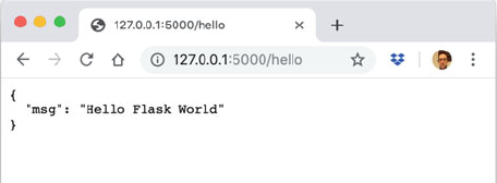
40.6.6 Invoking the Service

We will use a web browser to access the web service. To do this we must enter the full

URL that will route the request to our running appli cation and to the welcome()

function.

The URL is actually comprised of two elements, the ﬁrst part is the machine on

which the application is running and the port that it is using to listen for requests.

This is actually listed in the above output—look at the line starting ‘Running on’.

This means that the URL must start with http://127.0.0.1:5000. This

indicates that the application is running on the computer with the IP address

127.0.0.1 and listening on port 5000.

We could of course also use localhost instead of 127.0.0.1.

The remainder of the URL must then provide the information that will allow

Flask to route from the computer and port to the functions we want to run.

Thus the full URL is http://127.0.0.1:5000/hello and thus is used in

the web browser shown below:

As you can see the result returned is the text we supplied to the jsonify()

function but now in plain JSON format and displayed within the Web Browser.

You should also be able to see in the console output that a request was received

by the Flask framework for the GET request mapped to the /hello URL:

127.0.0.1 - - [23/May/2019 11:09:40] "GET /hello HTTP/1.1" 200

One useful featu re of this approach is that if you make a change to your program

then the Flask framework will notice this change when running in development

mode and can restart the web service with the code changes deployed. If you do this

you will see that the output notiﬁes you of the change:

* Detected change in 'hello_flask_world.py', reloading

* Restarting with stat

This allows changes to be made on the ﬂy and their effect can be immediately

seen.

478 40 Web Services in Python

40.6.7 The Final Solution

We can tidy this example up a little by deﬁning a function hat can be used to create

the Flask application object and by ensuring that we only run the application if

the code is being run as the main module:

from flask import Flask, jsonify, url_for

def create_service():

app = Flask(__name__)

@app.route('/hello', methods=['GET'])

def welcome():

return jsonify({'msg': 'Hello Flask World'})

with app.test_request_context():

print(url_for('welcome'))

return app

if __name__ == '__main__':

app = create_service()

app.run(debug=True)

One feature we have added to this program is the use of the test_re-

quest_context(). The test request context object returned implements the

context manager protocol and thus can be used via a with statement; this is useful

for debugging purposes. It can be used to verify the URL used for any functions

with routing information speciﬁed. In this case the output from the print statement is

‘/hello’ as this is the URL deﬁned by the @app.route decorator.

40.7 Online Resources

See the following online resources for information on the topics in this chapter:

•

http://www.ics.uci.edu/*ﬁelding/pubs/dissertation/top.htm Roy Fieldings’

Ph.D. Thesis; if you are interesting in the background to REST read this.

•

https://wiki.python.org/moin/WebFrameworks for a very extensive list of web

frameworks for Python.

•

https://www.djangoproject.com/ for information on Django.

•

http://www.web2py.com/ Web2py web framework documentation.

•

https://cherrypy.org/ For documentation on the CherryPy web framework.

•

http:// ask.pocoo.org/ For information and examples on the Flask web devel-

opment framework.

40.6 Hello World in Flask 479

• http:// ask.pocoo.org/docs/1.0/foreword/#what-does-micro-mean Flasks expla-

nation of what micro means.

•

https://www.json.org/ Information on JSON.

•

https://en.wikipedia.org/wiki/Web_Server_Gateway_Interface WSGI Web

Server Gateway Interface standard.

•

https://curl.haxx.se/ Infor mation on the curl command line tool.

•

https://developer.mozilla.org/en-US/docs/Web/HTTP/Status HTTP Response

Status Codes.

480 40 Web Services in Python

Chapter 41

Bookshop Web Service

41.1 Building a Flask Bookshop Service

The previous chapter illustrated the basic structure of a very simple web service

application. We are now in a position to explore the creation of a set of web services

for something a little more realistic; the bookshop web service application.

In this chapter we will implement the set of web services described earlier in the

previous chapter for a very simple bookshop. This means that we will deﬁne

services to handle not just the GET requests but also PUT, POST and DELETE

requests for the RESTful bookshop API.

41.2 The Design

Before we look at the implementation of the Bookshop RESTful API we will

consider what elements we for the services services.

One question that often causes some confusion is how web services relate to

traditional design approaches such as object oriented design. The approach adopted

here is that the Web Service API provides a way to implement an interface to

appropriate functions, objects and methods used to implement the application/

domain model.

This means that we will still have a set of classes that will represent the

Bookshop and the Books held within the bookshop. In turn the functions imple-

menting the web services will access the bookshop to retrieve, modify, update and

delete the books held by the bookshop.

J. Hunt, Advanced Guide to Python 3 Programming,

Undergraduate Topics in Computer Science,

https://doi.org/10.1007/978-3-030-25943-3_41

481

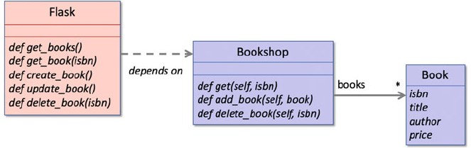
The overall design is shown below:

This shows that a Book object will have an isbn, a title, an author and a price

attribute.

In turn the Bookshop object will have a books attribute that will hold zero or

more Books. The books attribute will actually hold a List as the list of books

needs to change dynamically as and when new books are added or old books

deleted.

The Bookshop will also deﬁne three methods that will

• allow a book to be obtained via its isbn,

• allow a book to be added to the list of books and

• enable a book to be deleted (based on its isbn).

Routing information will be provided for a set of functions that will invoke

appropriate methods on the Bookshop object. The functions to be decorated with

@app.route, and the mappings to be used, are listed below:

• get_books() which maps to the /book/list URL using the HTTP Get

method request.

• get_book(isb n) which maps to the /book/<isbn> URL where isbn is a

URL parameter that will be passed into the function. This will also use the

HTTP GET request.

• create_book( ) which maps to the /book URL using the HTTP Post

request.

• update_book( ) which maps to the /book URL but using the HTTP Put

request.

• delete_book( ) which maps to the /book/<isbn> URL but using the

HTTP Delete request.

41.3 The Domain Model

The domain model comprises the Book and Bookshop classes. These are pre-

sented below.

482 41 Bookshop Web Service

The Book class is a simple Value type class (that is it is data oriented with no

behaviour of its own):

class Book:

def __init__(self, isbn, title, author, price):

self.isbn = isbn

self.title = title

self.author = author

self.price = price

def __str__(self):

return self.title + ' by ' + self.author + ' @ ' +

str(self.price)

The Bookshop class holds a list of books and provides a set of methods to

access books, update books and delete books:

class Bookshop:

def __init__(self, books):

self.books = books

def get(self, isbn):

if int(isbn) > len(self.books):

abort(404)

return list(filter(lambda b: b.isbn == isbn,

self.books))[0]

def add_book(self, book):

self.books.append(book)

def delete_book(self, isbn):

self.books = list(filter(lambda b: b.isbn != isbn,

self.books))

In the above code, the books attribute holds the list of books currently

available.

The get() method returns a book given a speciﬁed ISBN.

The add_book() method adds a book object to the list of books.

The delete_book() method removes a book based on its ISBN.

The bookshop global variable holds the Bookshop object initialised with a

default set of books:

41.3 The Domain Model 483

41.4 Encoding Books Into JSON

One issue we have is that although the jsonify() function knows how to convert

built in types such as strings, integers, lists, dictionaries etc. into an appropriate

JSON format; it does not know how to do this for custom types such as a Book.

We there fore need to deﬁne some way of converting a Book into an appropriate

JSON format.

One way we could do this would be to de ﬁne a method that can be called to

convert an instance of the Book class into a JSON format. We could call this

method to_json(). For example:

class Book:

""" Represents a book in the bookshop"""

def __init__(self, isbn, title, author, price):

self.isbn = isbn

self.title = title

self.author = author

self.price = price

def __str__(self):

return self.title + ' by ' + self.author + ' @ ' +

str(self.price)

def to_json(self):

return {

'isbn': self.isbn,

'title': self.title,

'author': self.author,

'price': self.price

}

We could now use this with the jsonify() function to convert a book into the

JSON format:

jsonify({'book': book.to

json()})

bookshop = Bookshop(

[Book(1, 'XML', 'Gryff Smith', 10.99),

Book(2, 'Java', 'Phoebe Cooke', 12.99),

Book(3, 'Scala', 'Adam Davies', 11.99),

Book(4, 'Python', 'Jasmine Byrne', 15.99)])

484 41 Bookshop Web Service

This approach certainly works and provides a very lightweight way to convert a

book into JSON.

However, the approach presented above does mean that every time we want to

jsonify a book we must remember to call the to_json() method. In some cases

this means that we will also have to write some slightly convoluted code. For

example if we wish to return a list of books from the Bookshop as a JSON list we

might write:

jsonify({'books': [b.to

json() for b in bookshop.books]})

Here we have used a list comprehension to generate a list containing the JSON

versions of the books held in the bookshop.

This is starting to look overly complex, easy to forget about and probably error

prone.

Flask itself uses encoders to encode types into JSON. Flask provides a way of

creating you r own encoders that can be used to convert a custom type, such as the

Book class, into JSON. Such an encoder can automatically be used by the jso-

nify() function.

To do this we must implement an encoder class; the class will extend the ﬂask.

json.JSONEncoder superclass.

The class must deﬁne a method default(self, obj).

This method takes an object and returns the JSON representation of that object.

We can therefore write an encoder for the Book class as follows:

The default() method in this class checks that the object passed to it is an

instance of the class Book and if it is then it will create a JSON version of the

Book. This JSON structure is based on the isbn, title, author and price attributes. If

it is not an instance of the Book class, then it passes the object up to the parent

class.

We can now register this encoder with the Flask application object so that it will

be used whenever a Book must be converted into JSON. This is done by assigning

the custom encoder to the Flask application object via the app.json_encoder

attribute:

class BookJSONEncoder(JSONEncoder):

def default(self, obj):

if isinstance(obj, Book):

return {

'isbn': obj.isbn,

'title': obj.title,

'author': obj.author,

'price': obj.price

}

else:

return super(BookJSONEncoder, self).default(obj)

41.4 Encoding Books Into JSON 485

Now if we wish to encode a single book or a list of books the above encoder will

be used automatically and thus we do not need to do anything else. Thus our earlier

examples can be written to simply by referencing the book or bookshop.books

attribute:

jsonify({'book': book})

jsonify({'books': bookshop.books})

41.5 Setting Up the GET Services

We can now set up the two services that will support GET requests, these are the

• /book/list and /book<isbn> services.

The functions that these URLs map to are given below:

def get_books():

return jsonify({'books': bookshop.books})

@app.route('/book/<int:isbn>', methods=['GET'])

def get_book(isbn):

book = bookshop.get(isbn)

return jsonify({'book': book})

@app.route('/book/list', methods=['GET'])

The ﬁrst function merely returns the current list of books held by the bookshop

in a JSON structure using the key books.

The second function takes an isbn number as parameter. This is a URL

parameter; in other words part of the URL used to invoke this function is actually

dynamic and will be passed into the function. This means that a user can request

details of books with different ISBNs just by changing the ISBN element of the

URL, for example:

• /book/1 will indicate that we want information on the book with the ISBN 1.

• /book/2 will indicate we want information on the book with ISBN 2.

In Flask to indicate that something is a URL parameter rather than a hard coded

element of the URL, we use angle brackets (<>). These surround the URL

parameter name and allow the parameter to be passed into the function (using the

same name).

app = Flask(__name__)

app.json_encoder = BookJSONEncoder

486 41 Bookshop Web Service

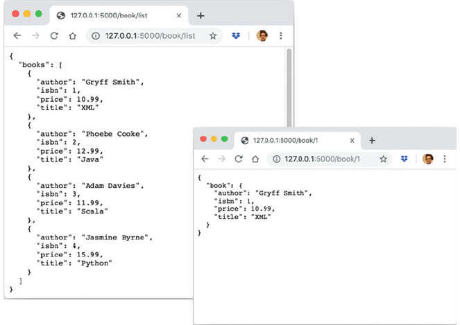
In the above example we have also (optionally) indicated the type of the

parameter. By default the type will be a string; however we know that the ISBN is

in fact an integer and so we have indicated that by preﬁxing the parameter name

with the type int (and separated the type information from the parameter name by a

colon ‘:’). There are actually several options available incl uding

• string (the default),

• int (as used above),

• ﬂoat for positive ﬂoating point values,

• uuid for uuid strings and

• path which dislike string but accepts slashes.

We can again use a browser to view the results of calling these services; this time

the URLs will be

• http://127.0.0.1:5000/book/list and

• http:/127.0.0.1:5000/book/1

for example:

As you can see from this the book information is returned as a set of key/value

pairs in JSON format.

41.5 Setting Up the GET Services 487

41.6 Deleting a Book

The delete a book web service is very similar to the get a book service in that it

takes an isbn as a URL path parameter. However, in this case it merely returns an

acknowledgement that the book was deleted successfully:

@app.route('/book/<int:isbn>', methods=['DELETE'])

def delete_book(isbn):

bookshop.delete_book(isbn)

return jsonify({'result': True})

However, we can no longer test this just by using a web browser. This is because

the web browser uses the HTTP Get request method for all URLs entered into the

URL ﬁeld. However, the delete web service is associated with the HTTP Delete

request method.

To invoke the delete_book() funct ion we therefore need to ensure that the

request that is sent uses the DELETE request method. This can be done from a

client that can indicate the type of request method being used. Examples might

include another Python program, a JavaScript web site etc.

For testing purposes, we will however use the curl program. This program is

available on most Linux and Mac systems and can be easily installed, if it is not

already available, on other operating systems.

The curl is a command line tool and library that can be used to send and

receive data over the internet. It supports a wide range of protocols and standards

and in particular supports HTTP and HTTPS protocols and can be used to send and

receive data over HTTP/S using different request methods.

For examp le, to invoke the delete_book() function using the /book/2

URL and the HTTP Delete method we can use curl as follows:

curl http://localhost:5000/book/2 -X DELETE

This indicates that we want to invoke the URL (http://localhost:5000/book/2)

and that we wish to use a custom request method (i.e. Not the default GET) which is

in the case DELETE (as indicated by the −X option). The result returned by the

command is given below indicating that the book was successfully deleted.

{

"result": true

}

We can verify this by checking the output from the /book/list URL in the

web browser:

488 41 Bookshop Web Service

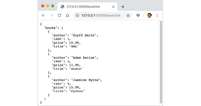
This conﬁrms that book 2 has been deleted.

41.7 Adding a New Book

We also want to support adding a new book to the Bookshop. The details of a new

book could just be added to the URL as URL path parameters; however as the

amount of data to be added grows this would become increasingly difﬁcult to

maintain and verify. Indeed although historically there was a limit of 2083 char-

acters in Microsoft’s Internet Explore (IE) which has theoretically be removed since

IE8, in practice there are typically still limits on the size of the URL. Most web

servers have a limit of 8 KB (or 8192 bytes) although this is typically con ﬁgurable.

There may also be client side limits (such as those imposed by IE or Apple’s Safari

(which usually have a 2 KB limit). If the limit is exceeded in either a browser or on

the server, then most systems will just truncate the characters outside the limit (in

some cases without any warning).

Typically such data is therefore sent in the body of the HTTP request as part of a

HTTP Post request. This limit on the same of a Post requests message body is much

higher (usually up to 2 GB). This means that it is a much more reliable and safer

way to transfer data to a web service.

However, it should be noted that this does not mean that the data is any more

secure than if it is part of the URL; just that it is sent in a different way.

From the point of view of the Python functions that are invoked as the result of a

HTTP Post method request it means that the data is not available as a parameter to

41.6 Deleting a Book 489

the URL and thus to the function. Instead, within the funct ion it is necessary to

obtain the request object and then to use that to obtain the information held within

the body of the request.

A key attribute on the request object, available when a HTTP request contains

JSON data, is the request.json attribute. This attribute contains a dictionary

like structure holding the values associated with the keys in the JSON data

structure.

This is shown below for the create_book() function.

from flask import request, abort

@app.route('/book', methods=['POST'])

def create_book():

print('create book')

if not request.json or not 'isbn' in request.json:

abort(400)

book = Book(request.json['isbn'],

request.json['title'],

request.json.get('author', ""),

float(request.json['price']))

bookshop.add_book(book)

return jsonify({'book': book}), 201

The above function accesses the ﬂask.request object that represents the

current HTTP request. The function ﬁrst checks to see that it contains JSON data

and that the ISBN of the book to add, is part of that JSON structure. If it the ISBN is

not then the ﬂask.abort() function is called passing in a suitable HTTP

response status code. In this case the error code indicates that this was a Bad

Request (HTTP Error Code 400).

If however the JSON data is present and does contain an ISBN number then the

values for the keys isbn, title, author and price are obtained. Remember

that JSON is a dictionary like structure of keys and values thus treating it in this

way makes it easy to extra ct the data that a JSON structure holds. It also means that

we can use both method and key oriented access styles. This is shown above where

we use the get() method along with a default value to use, if an author is not

speciﬁed.

Finally, as we want to treat the price as a ﬂoating point number we must use the

ﬂoat() function to convert the string format supplied by JSON into a ﬂoat.

Using the data extracted we can instantiate a new Book instance that can be

added to the bookshop. As is common in web services we are returning the newly

created book object as the result of creating the book along with the HTTP response

status code 201, which indicates the successful creation of a resource.

490 41 Bookshop Web Service

We can now test this service using the curl command line program:

curl -H "Content-Type: application/json" -X POST -d

'{"title":"Read a book", "author":"Bob","isbn":"5",

"price":"3.44"}' http://localhost:5000/book

The options used with this command indicate the type of data being sent in the

body of the request (-H) along with the data to include in the body of the request ( -

d). The result of running this command is:

{

"book": {

"author": "Bob",

"isbn": "5",

"price": 3.44,

"title": "Read a book"

}

Illustrating that the new book by Bob has been added.

41.8 Updating a Book

Updating a book that is already held by the bookshop object is very similar to

adding a book except that the HTTP Put request method is used.

Again the function implementing the required behaviour must use the ﬂask.

request object to access the data submitted along with the PUT request.

However, in this case the ISBN number speciﬁed is used to ﬁnd the book to be

updated, rather than the specifying a completely new book.

The update_book() function is given below:

@app.route('/book', methods=['PUT'])

def update_book():

if not request.json or not 'isbn' in request.json:

abort(400)

isbn = request.json['isbn']

book = bookshop.get(isbn)

book.title = request.json['title']

book.author = request.json['author']

book.price = request.json['price']

return jsonify({'book': book}), 201

41.7 Adding a New Book 491

This function resets the title, author and price of the book retrieved from

the bookshop. It again returns the updated book as the result of running the

function.

The curl program can again be used to invoke this function, although this time

the HTTP Put method must be speciﬁed:

curl -H "Content-Type: application/json" -X PUT -d

'{"title":"Read a Python Book", "author":"Bob

Jones","isbn":"5", "price":"3.44"}'

http://localhost:5000/book

The output from this command is:

{

"book": {

"author": "Bob Jones",

"isbn": "5",

"price": "3.44",

"title": "Read a Python Book"

}

This shows that book 5 has been updated with the new information.

41.9 What Happens if We Get It Wrong?

The code presented for the bookshop web services is not particularly defensive, as it

is possible to try to add a new book with the same ISB N as an existing one.

However, it does check to see that an ISBN number has been supplied with both the

create_book() and update_book() functions.

However, what happens if an ISBN numbe r is not supplied? In both functions

we call the ﬂask.abort() function. By default if this happens an error message

will be sent back to the client.

For example, in the following command we have forgotten to include the ISBN

number:

curl -H "Content-Type: application/json" -X POST -d

'{"title":"Read a book", "author":"Tom Andrews",

"price":"13.24"}' http://localhost:5000/book

492 41 Bookshop Web Service

This generates the following error output:

<!DOCTYPE HTML PUBLIC "-//W3C//DTD HTML 3.2 Final//EN">

<title>400 Bad Request</title>

<h1>Bad Request</h1>

<p>The browser (or proxy) sent a request that this server could

not understand.</p>

The odd thing here is that the error output is in HTML format, which is not what

we might have expected since we are creating a web service and working with

JSON. The problem is that Flask has default to generating an error HTML web page

that it expects to be rendered in a web browser.

We can overcome this by deﬁning our own custom error handler function. This

is a function that is decorated with an @app.errorhandler() decorator which

provides the response status code that it handles. For example:

@app.errorhandler(400)

def not_found(error):

return make_response(jsonify({'book': 'Not found'}), 400)

Now when a 400 code is generated via the ﬂask.abort() function, the

not_found() funct ion will be invoked and a JSON response will be generated

with the information provided by the ﬂask.make_response() function. For

example:

curl -H "Content-Type: application/json" -X POST -d

'{"title":"Read a book", "author":"Tom Andrews",

"price":"13.24"}' http://localhost:5000/book

The output from this command is:

{

"book": "Not found"

}

41.9 What Happens if We Get It Wrong? 493

41.10 Bookshop Services Listing

The complete listing for the bookshop web services application is given below:

from flask import Flask, jsonify, request, abort, make_response

from flask.json import JSONEncoder

class Book:

def __init__(self, isbn, title, author, price):

self.isbn = isbn

self.title = title

self.author = author

self.price = price

def __str__(self):

return self.title + ' by ' + self.author + ' @ ' +

str(self.price)

class BookJSONEncoder(JSONEncoder):

def default(self, obj):

if isinstance(obj, Book):

return {

'isbn': obj.isbn,

'title': obj.title,

'author': obj.author,

'price': obj.price

}

else:

return super(BookJSONEncoder, self).default(obj)

494 41 Bookshop Web Service

class Bookshop:

def __init__(self, books):

self.books = books

def get(self, isbn):

if int(isbn) > len(self.books):

abort(404)

return list(filter(lambda b: b.isbn == isbn,

self.books))[0]

def add_book(self, book):

self.books.append(book)

def delete_book(self, isbn):

self.books = list(filter(lambda b: b.isbn != isbn,

self.books))

bookshop = Bookshop([Book(1, 'XML', 'Gryff Smith', 10.99),

Book(2, 'Java', 'Phoebe Cooke', 12.99),

Book(3, 'Scala', 'Adam Davies', 11.99),

Book(4, 'Python', 'Jasmine Byrne', 15.99)])

def create_bookshop_service():

app = Flask(__name__)

app.json_encoder = BookJSONEncoder

@app.route('/book/list', methods=['GET'])

def get

books():

return jsonify({'books': bookshop.books})

@app.route('/book/<int:isbn>', methods=['GET'])

def get_book(isbn):

book = bookshop.get(isbn)

return jsonify({'book': book})

41.10 Bookshop Services Listing 495

@app.route('/book', methods=['POST'])

def create_book():

print('create book')

if not request.json or not 'isbn' in request.json:

abort(400)

book = Book(request.json['isbn'],

request.json['title'],

request.json.get('author', ""),

float(request.json['price']))

bookshop.add_book(book)

return jsonify({'book': book}), 201

@app.route('/book', methods=['PUT'])

def update_book():

if not request.json or not 'isbn' in request.json:

abort(400)

isbn = request.json['isbn']

book = bookshop.get(isbn)

book.title = request.json['title']

book.author = request.json['author']

book.price = request.json['price']

return jsonify({'book': book}), 201

@app.route('/book/<int:isbn>', methods=['DELETE'])

def delete_book(isbn):

bookshop.delete_book(isbn)

return jsonify({'result': True})

@app.errorhandler(400)

def not_found(error):

return make_response(jsonify({'book': 'Not found'}),

400)

return app

if __name__ == '__main__':

app = create_bookshop_service()

app.run(debug=True)

496 41 Bookshop Web Service

41.11 Exercises

The exercises for this chapter involves creating a web service that will provide

information on stock market prices.

The services to be implemented are:

Get method:

• /stock/list this will return a list of the stocks that can be queried for their

price.

• /stock/ticke r this will return the current price of the stock indicated by

ticker, for example/stock/APPL or/stock/MSFT.

POST method:

• /stock with the request body containing JSON for a new stock tick er and

price, for example {‘IBM’: 12.55}.

PUT method:

• /stock with the request body containing JSON for an existing stock ticker and

price.

DELETE method

• /stock/<tick er> which will result in the stock indicated by the ticker

being deleted from the service.

You could initialise the service with a default set of stocks and prices such as

[('IBM', 12.55), ('APPL', 15.66), ('GOOG', 5.22)].

You can test these services using the curl command line tool.

41.11 Exercises 497